Symptoms, signs and statistics

Experimental determination or detection of the physiological mechanisms underlying disease is by and large a highly complex task. This fact has turned epidemiology into the main tool for generating knowledge in the medical field. Epidemiology studies diseases by monitoring the health of groups of people, rather than through individual observations. If the primary tool for generating medical knowledge is based on the observation of groups of people (population samples) from which we wish to learn (make inferences), then the link between statistics and medicine is clear. Here we illustrate this nexus presenting three statistical research areas that are particularly valuable for biomedical research.

Keywords: biostatistics, health and life sciences, clinical trials, epidemiology, survival.

Epidemiology and spatial statistics

It is very common to find towns where people believe that their health is worse than the health of the surrounding municipalities. For some reason their inhabitants think their chances of dying, due to one or many specific causes, are higher compared to those of the inhabitants of neighbouring towns. Giving an adequate response to such a belief entails a great statistical complexity that is difficult to foresee given the simplicity of the question at hand.

«Epidemiology tries to identify the links between the presence of both risk factors and diseases in specific population groups»

Epidemiology attempts to identify the links between the presence of both risk factors and diseases in specific population groups. This task is «relatively» simple at a population level; it is all about getting the appropriate sample with the required amount of participants. However, focusing on population samples rather than individuals has made epidemiology a unique discipline within medicine and the main generator of knowledge regarding diseases. One of the risk factors historically studied is the geographic location of people; i.e. whether or not this can have an influence on the presence of a specific disease. Establishing this relationship can be very useful for medical professionals, because it can provide some possibly unknown clues that some characteristic of a particular region might have an influence on the risk of developing a specific disease.

«Disease mapping is
a clear example of the symbiosis between statistics and medicine»

However, when studying the relationship between geographical locations and the presence of a certain disease the size of the unit of study is of great relevance. Obviously, someone who suspects that his or her town has a high mortality rate due to some specific disease will not just be content knowing that, taking into account the whole region, the mortality rate is within reasonable parameters. In addition, working with large units of study means that an exceptional increase of the risk in a very specific location may be blurred by the regular risk in the rest of the unit. Consequently, it is advisable to work with the smallest geographic units possible in order to conduct studies of this kind. However, working with small geographic units affords limited information. As a result, problems that require the use of appropriate statistical techniques for this specific type of situation arise.

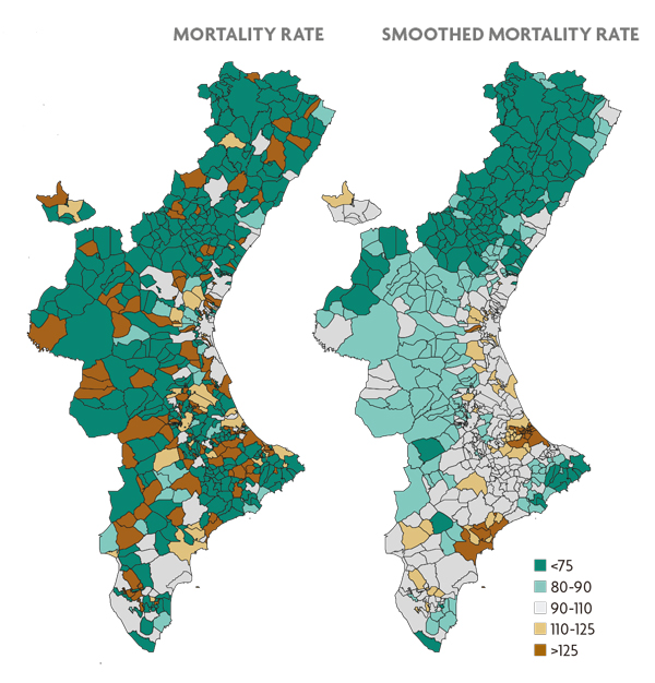
Figure 1. Estimation of the mortality risk due to oral cavity and pharynx cancer for the municipalities of the Valencian Community. The map on the left reflects the estimate obtained by the standardised mortality ratio, an indicator frequently used in epidemiology. The map on the right employs the same estimate obtained from Besag, York and Mollie’s statistical model. In both maps brown municipalities represent locations with higher risk in contrast with those depicted in green.

The mortality rates we are referring to, from an epidemiological perspective, would be calculated as the result of dividing the actual number of deaths between the expected number in each municipality based on its size and the composition of its population and multiplying it by 100. This indicator is known as the standardised mortality ratio (or rate). If this ratio is greater than 100 (respectively less) in a specific geographic location, this would indicate that there have been more (respectively less) deaths than would be expected given the size of its population, i.e. the location has risk excess. When working with small geographical units, the number of expected deaths will be, in turn, very small. Therefore, the ratio above will be either 0, if there have not been any deaths in the population, or a number considerably higher than 100, in the opposite case. So, if we use these rates, small municipalities will necessarily show extreme mortality rates, simply because of their size, regardless of the risk they might be associated with. We can visualise this in the map shown in Figure 1, which corresponds to the mortality caused by oral cancer in each municipality of the region of the Valencian Community. This figure shows that the inland areas of the provinces of Castellón and Valencia (the least populated areas of the Valencian Community) always present extreme rates, which does not mean that the risk in those areas is necessarily high or low.

Fortunately, statistics offers epidemiology inference tools that help to solve this problem. A number of models that consider the risks of municipalities as interdependent values have been proposed, in opposition to the standardised mortality ratio, which assumes such values as independent quantities. In particular, it is generally considered that the risks of neighbouring towns tend to be similar, unlike the risks of municipalities that are further away (Besag et al., 1991). This assumption makes it possible for neighbouring towns to share information with each other and thus we can obtain more solid estimates of these risks based on a greater amount of information (regarding each town and their neighbours). The right-hand map of Figure 1 shows the distribution of mortality estimated with a statistical model of the kind mentioned above, using the same data as in the left-hand map of the same figure. The smaller municipalities no longer seem to behave in any particular manner, and have more or less neutral values. Only the towns and surrounding areas with statistically sound mortality figures display truly extreme risk values.

«Fortunately, statistics offers epidemiology inference tools that help to solve spatial problems»

The contribution of statistics has made the study of mortality, as well as other health indicators, in small areas a research field in itself known today as disease mapping. This field has made the geographical study of health to a very detailed level possible today and a large number of articles are constantly published on the subject. These studies provide interesting clues, hypotheses and knowledge about the diseases studied. Undoubtedly, disease mapping is a clear example of the symbiosis between statistics and medicine. On the one hand, medicine offers statistics a field where it can develop and become meaningful, while on the other hand, statistics provides medicine with technical tools to accomplish its specific goals.

Clinical trials and statistics

A clinical trial is an experimental research project that uses humans as experimental units in which to intervene actively in order to assess the safety and efficacy of the intervention. This intervention may consist of a new treatment, a vaccine or a diagnosis or early diagnosis technique, etc. Since it involves experimentation with human beings one must follow strict ethical criteria from the planning to the completion of the trial. These criteria are listed in the Declaration of Helsinki of the World Medical Association and in its subsequent amendments. Most of these ethical criteria have been transposed into current legislation in Spain, such as the SCO/256/2007 of 5 February on good clinical practise. As a result, a clinical trial can only be proposed when there is already some evidence regarding the safety and efficacy of the intervention to be assessed, evidence based on observational studies and preclinical trials. Such trials must be approved by an ethics committee and the patients enrolled must be voluntary, fully informed of any of the risks the test involves and aware that they can leave whenever they want.

Clinical trials have become a basic tool for medical research, since they are the most effective way to compare the effectiveness of a new treatment with the one currently in use (Cook and DeMets, 2008). This is so because observational studies can establish associations between risk factors and disease, but it cannot easily prove causality; that is, whether the observed effect can be directly attributed to the new treatment or not. According to Rubin’s causal model (Rubin, 1974; Holland, 1986), in order to demonstrate causality, one should, ideally, observe the response of individual patients to the new treatment, Y_T, and at the same time their response if they have not been treated or have received conventional treatment, Y_C. The difference between the two values, Y_T – Y_C, is the effect directly attributable to the new treatment in that individual and is known as the «Rubin causal effect»; the average population effect is the expected value of this difference, E (Y_T– Y_C), which can be estimated using the arithmetic mean of the differences obtained in the observed patients. However, it is impossible to observe at the same time and in the same patient the response with and without the treatment, both Y_T and Y_C. Only one of these responses can be observed: this is the «fundamental problem of causal inference».

«One of the risk factors that has been historically studied is the geographic location of people, i.e. whether or not this can have an influence on the presence of a specific disease»

An important result of the theory of probability, the linearity of the expected value, circumvents the fundamental problem of causal inference, since it states that E (Y_T – Y_C) = E (Y_T) – E (Y_C); that is, the population mean effect is the average response to treatment, E (Y_T), minus the average response to no treatment, E (Y_C), and these average responses can be estimated separately using two different patient groups or the same group of patients in two different time periods. However, separate estimation involves other potential difficulties, possible sources of bias, which need to be avoided. Particularly, we must ensure that the two samples used to estimate the E (Y_T) and E (Y_C) effects separately are representative of the same population; we cannot treated patients to have some feature that differentiates them from the untreated ones. The easiest way to ensure this representativity in the same population is by recruiting patients first and thereafter assigning each patient to either the treated or the untreated group by means of any external random mechanism, e.g. tossing a coin. This is only possible in a study in which there is active intervention of the research team, as occurs in a clinical trial, but not in an observational study.

The clinical trial is prospective if there is follow-up of the enrolled patients in the near future, which can last for days, months or even years. The clinical trial is controlled if there are at least two groups of patients; the new treatment is applied to a patient group called «treatment group» and another treatment, frequently the most widely used at the time, is applied to another group of patients known as the «control group». There can be multiple treatment groups if we want to compare several treatments or therapeutic procedures. The trial is concurrent if all groups are recruited and observed simultaneously. It is randomised if the allocation of each patient to one of the groups is done at random; tossing a coin is an option, but more sophisticated procedures that use pseudo-random numbers, which enable the repetition of the process in a possible audit, are generally employed. If the trial is prospective, controlled, concurrent and randomised, it will meet the requirements of Rubin’s causal model, making it possible to demonstrate causality. This type of study should be used whenever possible (Matthews, 2006). Furthermore, to avoid bias among patients and health professionals when evaluating the effect of the treatment, we strongly advise the trial be made a double blind one: neither the patient nor the health professionals monitoring and evaluating should know the allocation of each patient.

The calculation of the sample size for the trial – the number of patients who take part in it – must also be determined in advance for ethical reasons. If the size of the sample is too small, it will provide too little information, so there will be very little chance of obtaining interesting results. This is not justifiable ethically, as patients will be put at risk with little or no guarantees of the trial being useful. Conversely, if the sample size is too large, more patients than needed will be exposed to an inferior treatment, which is not ethically justified either. To calculate an appropriate sample size power functions are usually used.

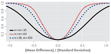
Figure 2. Power functions in a Student’s t-test to compare the means of two populations, using designs with different sample sizes, assuming equal variances and a significance level of α = 0.05; n and m are the sizes of each of the two samples.

Power functions calculate the probability of results being able to determine if there are differences between the study groups depending on the real magnitude of this difference. The power function at zero value should be small, since this is the probability of drawing a wrong conclusion when finding differences between groups when in fact there are none. It usually needs to be smaller or equal to α = 0.05. At nonzero values, this function provides the probability of correctly concluding that there are differences, so in these cases it should be as large as possible. The sample size is obtained by establishing a reasonable distance between the effects of the groups we are comparing and the power to be reached from that distance.

Figure 2 shows three power functions typically used to compare two means, the «Student’s t-test». These functions correspond to a significance value of α = 0.05, so they take this value at zero, which is the point that represents the null hypothesis of equal means. The dashed vertical line marks a distance between them of 0.5 standard deviation; at that distance and using 40 pieces of data, 20 in each group, we can only obtain a power of 0.35, which is too small a value. Using 128 pieces of data, 64 in each group, we obtain a power of 0.8. If we use 128 pieces of data, but distribute 28 in one group and 100 in the other, a lower power is obtained if compared to the results we would get if the groups had the same sample size. This is why it is advisable that the sample size of the groups remains the same.

Statistics provides the field of medicine with statistical inference methods that analyse the final results of the clinical trial and lead us to draw conclusions. Many of these methods are also widely used in other fields of knowledge, while others have been developed specifically in the context of health and life sciences, such as statistical survival methods and longitudinal models. Moreover, statistics also provide experimental design methodology that may prove very useful when planning the trial, helping to avoid bias and providing tools for the calculation of the sample size.

Survival statistics and longitudinal studies

Survival analysis (Aalen et al., 2008) is the statistical methodology specialised in analysing data that correspond to the elapsed time between two events – the initial event and the event of interest – in scientific studies in health sciences and biology. This time is generally known as survival time, a name inherited from the prototypical event of interest, death, common in early studies on the subject and that will be used in a general manner in this paper.

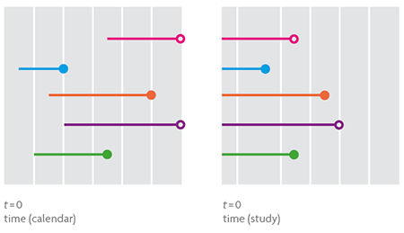
Figure 3. The graph on the left shows five survival times in real time, from entry in the study until departure, representing when the event of interest (small coloured dot) or censored survival (white dot). The graph on the right contains the same information explained above but time is now according to the scale of the study, with a starting time common to all individuals, which determines their entry into the study. This would be the appropriate scale in the case of a hypothetical statistical analysis of the data.

Survival analysis applied to non-biological contexts is known as reliability analysis. So when it comes to studying the lifetime of a person from birth to death, the time elapsed from infection with human immunodeficiency virus (HIV) to a diagnosis of acquired immunodeficiency syndrome (AIDS) or the survival of the red palm weevil after infesting a palm, we are talking about survival analysis. If, on the contrary, the goal is to analyse the time from start-up to failure of the cooling system at a nuclear power plant, the time between consecutive earthquakes in the Gulf of Valencia or how long the mosaic facade of a public building lasts, we are talking about reliability analysis.

To observe a survival time one must wait until the event of interest occurs. This situation is hardly feasible in survival studies because its duration is usually limited and, in most cases, the study concludes with no event of interest observed in any of the individuals from the sample. Thus, the resulting data will contain the entire duration of survival of individuals for whom the event is registered as well as the incomplete survival, censored on the right, of individuals who «are still alive» at the end of the study. The existence of censored data in a survival study makes its analysis through traditional statistical methods impossible (Figure 3).

The survival function and the risk function are basic concepts of survival analysis. The former allows us to estimate probabilities associated with specific moments in time, such as a person diagnosed with colon cancer surviving over five years. The risk function is a rate and as such quantifies, for example, the risk of death in people who have undergone a delicate surgical procedure, usually decreasing as the postoperative period lengthens.

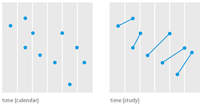
Figure 4. Statistical models to analyse longitudinal data are complex but also very powerful, because they are able to quantify not only the general evolution of the variable of interest in the target population, but also the specific progression of any individual or group of relevant individuals. The graph on the left shows some data in which the observations regarding the same individual are unidentified, while the one on the right shows data regarding the same individual connected by a segment. The first one shows a decreasing ratio over time; the second shows the opposite.

Not all people face situations the same way others do, much less regarding mortality and morbidity issues. Survival times associated with an event are often related to a set of risk variables whose values can help us understand the different survival times of different individuals within a population a little better. For example, it is known that a person with high levels of cholesterol has a higher risk of presenting cardiovascular problems than a person with lower levels. The Cox regression models and the so-called accelerated lifetime models let us model the survival function as well as the risk function using these variables, both when they can and cannot be observed or have not been registered, in the knowledge that heterogeneity is a possibility. We can quantify their importance in terms of probability, the natural language of statistics, thanks to statistical inference, and to Bayesian methodology in particular.

Cross-sectional studies collect information from sampled individuals at a single, very specific point in time. They are fast running and generally inexpensive. Longitudinal studies (Diggle et al., 2002), based on repeated measurements of the same individual over time, are costly and slow because, like survival studies, they require extended periods of observation (Figure 4). They are particularly important in the epidemiological studies of chronic diseases (Alzheimer’s disease, asthma, cancer, diabetes, cardiovascular and renal diseases, AIDS, etc.), the main cause of mortality in the world and responsible for about 60 % of all deaths.

The origins of longitudinal models date back to the early nineteenth century with the pioneering work of the English mathematician George Biddel Airy (1801-1892) in the field of astronomy. Their popularisation in the world of statistics has come about with the great computational developments of the mid and late twentieth century, which have enabled their practical implementation and subsequent use in the statistical treatment of socially relevant scientific problems, such as research on the relationship between the CD4 cell count and the viral load as a marker of the progression of HIV infection.

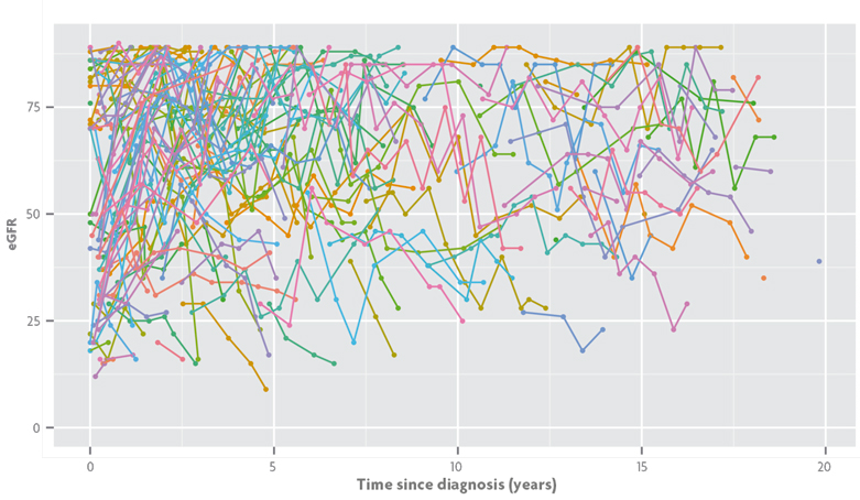
Figure 5. Estimated glomerular filtration rate (eGFR) for a longitudinal study on the progression of chronic renal failure in Valencian children. EGFR levels are represented in the time scale arising from the diagnosis of the disease and different consecutive eGFR measurements for the same child appear connected by segments of the same colour. / Data from Isabel Zamora, María José Sanahuja and Silvia Agustí.

Returning to survival studies, as we await the occurrence of the event of interest, we can conduct a longitudinal follow-up of the relevant variables in the study and incorporate the information to the survival model. This idea is the genesis of the so-called joint models for survival and longitudinal data. When, as in the case described, the aim of the study focuses solely on survival, longitudinal models provide valuable information for the survival model, such as longitudinal measurements of prostate-specific antigen (PSA) in prostate cancer studies. Joint models, however, are more powerful because they make equal treatment between the two processes possible and enable the use of survival analysis tools in simple longitudinal studies. In this sense, the data in Figure 5 corresponds to a longitudinal study on the progression of chronic renal failure in Valencian children. The variable of interest is the estimated glomerular filtration rate (eGFR), which decreases as renal function worsens and provides information regarding the values that mark the different stages of the disease. During the follow-up period some children leave the study and we do not get the complete longitudinal information. If the reason for leaving the study is related to disease progression it is convenient to add this information to the longitudinal model. In our case, it is the children who are temporarily cured (their eGFR gradually increases until their medical discharge) or those that suffer a critical worsening of their renal function and require renal replacement therapy (dialysis or transplant). By using joint models we can incorporate this information into a longitudinal analysis through a survival model that considers the need for renal replacement therapy and healing as events of interest, which are naturally incompatible.

References

Aalen, O. O.; Borgan, Ø. and H. K. Gjessing, 2008. Survival and Event History Analysis: A Process Point of View. Springer. New York.
Besag, J.; York, J. and A. Mollié, 1991. «Bayesian Image Restoration, with Two Applications in Spatial Statistics». Annals of the Institute of Statistical Mathematics, 43(1): 1-20. DOI: <10.1007/BF00116466>.
Cook, T. D. and D. L. DeMets, 2008. Introduction to Statistical Methods for Clinical Trials. Chapman & Hall/CRC. Boca Raton, USA.
Diggle, P. J.; Heagerty, P. J.; Liang, K.-Y. and S. Zeger, 2002. Analysis of Longitudinal Data. Oxford University Press.
Oxford. Holland, P. W., 1986. «Statistics and Causal Inference». Journal of the American Statistical Association, 81(396): 945-960. DOI: <10.2307/2289064>.
Matthews, J. N. S., 2006. Introduction to Randomized Controlled Clinical Trials. Chapman & Hall/CRC. Boca Raton, USA.
Rubin, D. B., 1974. «Estimating Causal Effects of Treatments in Randomized and Non-Randomized Studies». Journal of Educational Psychology, 66 (5): 688-701. DOI: <10.1037/h0037350>.