Statistics in particle physics

Statistics has played a decisive role in the development of particle physics, a pioneer of the so-called «big science». Its usage has grown alongside technological developments, enabling us to go from recording a few hundred events to thousands of millions of events. This article discusses how we have solved the problem of handling these huge datasets and how we have implemented the main statistical tools since the 1990s to search for ever smaller signals hidden in increasing background noise. The history of particle physics has witnessed many experiments that could illustrate the role of statistics, but few can boast a discovery of such scientific impact and dimensions as the Higgs boson, resulting from a colossal collective and technological endeavour.

Keywords: Statistics, Monte Carlo, p-value, particle physics, Higgs boson.

«The principle of science, the definition, almost, is the following: The test of all knowledge is experiment. Experiment is the sole judge of scientific “truth”. But what is the source of knowledge? Where do the laws that are to be tested come from? Experiment, itself, helps to produce these laws, in the sense that it gives us hints. But also needed is imagination to create from these hints the great generalizations […], and then to experiment to check again whether we have made the right guess.» (Feynman, 1963). Thus, the great physicist Richard Feynman summed up the role of experimentation in scientific method. Nowadays, deep into the age of the generation and manipulation of massive amounts of data we know as Big Data, statistics is a fundamental tool for science. In genomics, climate change or particle physics, discoveries arise only when we analyse data through the prism of statistics, since the desired signal, if it exists, is hidden among a huge amount of background noise.

«Deep into the age
of the generation
and manipulation
of massive amounts
of data, statistics is
a fundamental tool for science»

Particle physics emerged as a distinct discipline towards the 1950s, pioneering «big science», as it required experiments with large particle accelerators and detectors and Big Data infrastructure, developed through large collaborations. In this environment statistics has played a role of great importance, although without strong ties to the statistical community, a situation that has significantly improved in recent years (Physics Statistics Code Repository, 2002, 2003, 2005, 2007, 2011).

Its field of study is the «elementary particles» that have been discovered and, together with the forces between them, form what is known as the standard model: 6 quarks (u, d, s, c, b, t); 6 leptons (electron, muon, tau and their associated neutrinos); intermediate bosons for fundamental interactions (the photon for electromagnetic interaction, two W and one Z for the weak, and the 8 gluons for the strong; gravitational interaction, much less intense, has not yet been satisfactorily included); and the two hundred hadrons consisting of two quarks (called mesons), three quarks (baryons) or even four quarks (tetraquarks, whose evidences are becoming more and more convincing; Swanson, 2013; Aaij et al., 2014). We must add to the list their corresponding antimatter pairs: antiquarks, antileptons and antihadrons. And, of course, the new Higgs boson, proof of the Englert-Brout-Higgs field that fills the void and is responsible for providing mass to all those particles (except photons and gluons, which do not have mass), discovered in 2012 after being postulated fifty years earlier (Schirber, 2013). We must add to all this what we have yet to discover, such as super-symmetric particles, dark matter, etc. The list is limited only by the imagination of the theorists who propose them. However, although the nature of this «new physics» is unknown, there are strong reasons that suggest their actual existence, so the search continues (Ellis, 2012).

The questions we need to answer for each kind of particle are varied: Does it exist? If it does, what are its properties (mass, spin, electric charge, mean lifetime, etc.)? If it is not stable, what particles are produced when it decays? What are the probabilities of the different decay modes? How are energies and directions of the particles distributed during their final state? Are they in accordance with our theoretical models? What processes occur, with which cross sections (probabilities), when it collides with another particle? Does its antiparticle behave the same way?

In order to study a particular phenomenon we need, first, to reproduce it «under controlled conditions». To that end, particle beams from an accelerator or from other origins such as radioactive sources or cosmic rays are often used, bombarding a fixed target or setting them against each other. The type and energy of the colliding particles are chosen to maximise the incidence of the particular phenomenon. In the «energy frontier» accelerators allow for higher energies in order to produce new particles, while in the «luminosity frontier», they can expose processes with major implications previously considered impossible or very rare.

Let’s consider the case of the Gran Col·lisionador d’Hadrons (LHC) del CERN in Geneva, which started working in 2009, after close to twenty years of design and construction. In this accelerator protons collide at an energy of up to 7 TeV per proton (1 TeV = a billion eVs). In everyday terms, 1 TeV is similar to the kinetic energy of a mosquito. What makes this energy so strong is that it is concentrated in a region the size of a billionth of a speck of dust. To record what happens after the collision large detectors have been built (ATLAS and CMS for studies on the energy frontier, LHCb and ALICE for the luminosity frontier, and other smaller ones) consisting of a wide array of sensors with millions of electronic reading channels.

Big Data

«In the LHC, some ultra-fast electronic systems called triggers decide in real time whether the collision is interesting or not. If so, it is recorded on hard disks to be reconstructed and analysed later»

In the LHC experiments beams collide 20 million times per second. Each of these collisions produces a small explosion in which part of the kinetic energy of the protons is converted into other particles. Most are very unstable and decay, producing a cascade of hundreds or thousands of lighter, more stable particles which are directly observable in the detectors. Using a few characteristics of these residues, some ultra-fast electronic systems called triggers decide in real time whether the collision is interesting or not. If so, it is recorded on hard disks to be reconstructed and analysed later. These data acquisition systems (Figure 1) reduce the collisions that are of relevance in terms of physics to a few hundred per second, generating approximately 1 petabyte (one thousand million megabytes) of «raw» data per year per experiment.

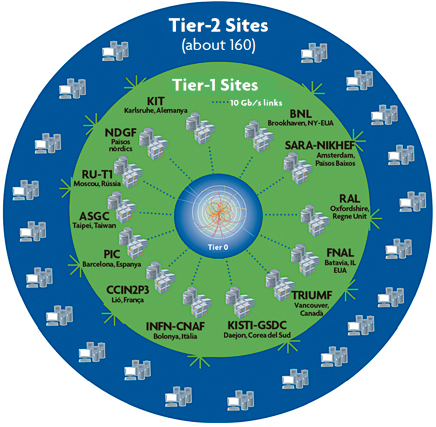
Figure 2. Diagram of the distribution of computer centres for LHC experiments. Tier-1 centres, spread across Asia, Europe and North America, are linked to Tier-0 at CERN using dedicated connections of up to 10 gigabits per second, while the Tier-1 and Tier-2 centres are interconnected using the research networks of each particular country. In turn, all Tier centres are connected to the general Internet. Thus, any Tier-2 centre can access every bit of data. The name of this data storage and mass calculation infrastructure is Worldwide LHC Computing Grid (WLCG). Tier-0 and Tier-1 are dedicated to (re)processing real data and to permanent storage of both real and simulated data. The raw data are stored only on Tier-0. Meanwhile, the Tier-2 centres are devoted to partial and temporary data storage, Monte Carlo productions and processing the final stages of data analysis. / WLCG Collaboration © 2014, http://wlcg.web.cern.ch

In the reconstruction phase electronic signals constituting raw data are combined and interpreted: the impacts left by particles passing through sensors allow their trajectories to be traced, their intersections are searched to identify the position of the collision and disintegration of unstable particles, the curvature of their paths within a magnetic field determines the momentum, the calorimeters measure the energy of the particles, etc. From this process of pattern recognition emerges the «event» reconstructed as a list of produced particles with their measured kinematic magnitudes (energy, momentum, position and direction) and, often, their identity. The LHC experiments have developed a storage and massive computation infrastructure named WLCG (Worldwide LHC Computing Grid) that allows the reconstruction of thousands of millions of events produced annually to be distributed to hundreds of thousands of processors all around the world (Figure 2).

Once the pattern of the studied phenomenon is known, during the analysis stage a classification or selection of events (signal to noise) is chosen using hypothesis-contrasting techniques. With the challenge of discriminating smaller and smaller signals, recent years have witnessed how methods for multivariate classification based on learning techniques have emerged and evolved (Webb, 2002). This would not have been possible without the significant progress made by the statistics community in combining classifiers and improving their performance. The relevant magnitudes are evaluated for the selected events using the kinematic variables associated to the detected particles. Then they are represented graphically, usually as a frequency diagram (histogram).

An example of this process of data reduction is illustrated in Figure 3. In the upper part is the histogram of the invariant mass of photon pairs that exceeded the trigger, the reconstruction and event classification as «candidates» to be Higgs bosons produced and disintegrated into two photons. The physical magnitude considered, in this case invariant mass, is calculated from the energy and direction of the photons measured by the calorimeter. The complete reconstruction of the collision that leads to one of these candidates is illustrated in Figure 4, in which we can clearly identify the two photons over the hundreds of paths reconstructed from other particles produced in the collision. If the two photons come, in fact, from the production and decay of a new particle, the histogram should show an excess of events located over continuous background noise, as indeed seems to be the case. It is when comparing this distribution with the theory that the statistical questions of interest arise: is there any evidence of the Higgs boson? What is the best estimate of its mass, production cross-section and probability of decay to the final state of two photons? Are these results consistent with the prediction of the standard model?

Statistics and Monte Carlo simulations

Every experiment in particle physics can be understood as an experiment in event counting. Thus, in order to observe a particle and measure its mass, a histogram like the one in Figure 3 is used, in which the number of events (N) for each invariant mass interval is random and determined by the Poisson distribution, with standard deviation √N (only in some particular cases using binomial or Gaussian statistics becomes necessary, without dealing with the large limit for N). This randomness, however, is not the result of a sampling error. It is, rather, related to the quantum nature of the processes.

The distributions predicted by the theory are usually simple. For example, angular distributions can be uniform or come from trigonometric functions, masses usually follow a Cauchy distribution (particle physicists call them Breit-Wigner), temporal distributions can be exponential or exponential modulated by trigonometric or hyperbolic functions. These simple forms are often modified by complex theoretical effects, and always by resolution, efficiency and background noise associated with the reconstruction of the event.

These distributions are generated using Monte Carlo simulations. First, the particles are generated following the initial simple distributions, and theoretical complications are included later. To this end, a number of generators have been developed with such exotic names as Herwig, Pythia and Sherpa, which provide a complete simulation of the dynamics of collisions (Nason and Skands, 2013). Secondly, the theoretical distributions are corrected for the detector response.
To do so, it is necessary to encode a precise virtual model of its geometry and composition in specific programs, the most sophisticated and widespread of which is Geant (Agostinelli, 2003). Thus, the simulation of the detector accounts for effects such as the interaction of particles with the materials they pass through, the angular coverage, the dead areas, the existence of defective electronic channels or the inaccuracies in the positioning of the devices.

«The simulated data allows a complete prediction of the distributions that follow the data. The simulated data are also essential for planning new experiments»

One of the fundamental problems of simulation at different stages is sampling with high efficiency and maximum speed the probability density functions that define distributions. Uniformly random number generators with a long or extremely long period are used. When it is possible to calculate the inverse of the cumulative function analytically, the probability function is sampled with specific algorithms. This is the case of some common functions such as exponential, Breit-Wigner or Gaussian functions. Otherwise the more general, less efficient Von Neumann method (acceptance-rejection) is used.

The simulated data is used to reconstruct the kinematic magnitudes with the same software used for the actual data, which allows a complete prediction of the distributions that follow the data. Due to their complexity and slowness of execution, simulation programs absorb similar or even higher computing and storage resources from WLCG infrastructure than those of the real data (Figure 2). The simulated data is also essential for planning new experiments.

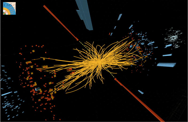
Figure 4. A candidate event to Higgs boson decaying into two photons whose energies deposited in the calorimeters of the detector are represented by red «towers». Yellow dotted straight lines illustrate the directions of photons, defined by the point of collision and the towers. Yellow solid lines represent the reconstructed paths of hundreds of other particles produced in the collision. The curvature of these paths allows measuring the time of the particles that produced them, and is due to the presence of an intense magnetic field. / CM Experiment © 2014 CERN

Estimating physical parameters and confidence intervals

Knowledge of the theoretical distributions, except for a few unknown parameters corrected by the measurement process, implies that the likelihood function is known and, therefore, it is possible to obtain their maximum likelihood estimators (Barlow, 1989; Cowan, 2013). Some examples of estimators that can be constructed from the distribution in Figure 3 would be the mass of the particle and the strength of the signal, the latter related to the output of the production cross section and the probability of decay of two photons. The corresponding regions of confidence for a given level of confidence are obtained from the variation in likelihood with regard to its maximum value. Very seldom is the solution algebraic, so numerical techniques are needed for complex problems with a large volume of data, which require significant computing resources. A traditional cheaper alternative is the least squares method, whereby an c²-type statistical test is minimised. Its main disadvantage lies in the assumption that the data follows a Gaussian distribution as an approximation to the Poisson distribution, so that, in general, there is a maximum likelihood estimator that is asymptotically efficient and unbiased. The binned method of maximum likelihood solves the issue by using Poisson likelihood for each interval instead of c². In this case the efficiency estimator is reduced only if the width of the intervals is higher than the data structure. The increased capacity of the processors and the advances in parallelisation protocols in recent years have allowed to implement the full maximum likelihood method.

During the last decade the use of the Toy Monte Carlo technique has also spread. This technique is also called «false experiments» for obtaining confidence regions using Neyman’s construction (Cowan, 2013). Taking the likelihood function as a starting point, data (false experiments) is generated for some specific values of the parameters. Each of these experiments is set to find the maximum likelihood estimator. Counting the number of experiments whose likelihood is lower or higher than the experimental likelihood, and exploring the parameter space, the confidence region with the desired confidence level is found. This technique is crucial when data is not well described by Gaussian distributions, and the likelihood is distorted with respect to its expected asymptotic behaviour or presents a local maximum close to the global maximum. It is also common to apply it in order to certify the probability content of confidence regions built with the Gaussian approximation.

Statistical significance and discovery

The probability that the result of an experiment is consistent with random data fluctuation when a hypothesis is true (referred to as a null hypothesis) is known as statistical significance or p-value (Barlow, 1989; Cowan, 2013): the lower it is, the greater the likelihood that the hypothesis is false. To calculate p, usually with the Toy Monte Carlo technique, we must define a data-dependent statistical test that reflects in some way the degree of discrepancy between the data and the null hypothesis. A typical implementation is the likelihood ratio between the best fitted data and the fit with the null hypothesis. Usually the p-value is converted into an equivalent significance Zσ, using the cumulative distribution of the normalized Gaussian distribution. Ever since the 1990s experiments in particle physics, scientists have been using a minimum criterion of 5σ, corresponding to a p-value of 2.87 × 10^-7, to conclusively exclude a null hypothesis. Only in this case can we speak about «observation» or «discovery». The criterion is about 3σ, with a p-value of 1.35 × 10^-3, for «evidence».

«The risk exists that the experimenter, ALBEIT unconsciously, monitors the experiment with the same data with which he made the observation, introducing changes, until they come to a desirable agreement»

These requirements are essential when measurements are subject to systematic uncertainty. Thus, in the early decades of the field of particle physics, experiments recorded, in the best of cases, hundreds of events, so statistical uncertainty was so high that systematic uncertainty was negligible. In the 1970s and 1980s, electronic detectors appeared and statistical uncertainty decreased. Nonetheless, great discoveries at the time, such as the b quark (Herb et al., 1977), with an observed signal of around 770 candidates on an expected number of events with the null hypothesis (noise) of 350, or the W boson by the UA1 experiment (Arnison et al., 1983), with 6 events observed over a negligible estimated noise, did not assess the level of significance of the findings. Nowadays, we have detailed analyses of such uncertainties, whose control requires, for example, calibrating millions of detector readout channels and carefully tuning the simulated data. A task which is complex in practise and generally induces non-negligible systematic uncertainty.

Figure 3. At the top is the distribution, shown as a histogram (points), of the invariant mass of the candidate events to Higgs bosons produced and disintegrated into two photons (Aad et al., 2012). This distribution is set by the maximum likelihood method to a model (solid red line) created from the sum of a signal function for a boson mass of 126.5 GeV (solid black line) and a noise function (dashed blue line). At the bottom is the distribution of data (dots) and fitted model (line) after subtracting the noise contribution. The quadratic sum of all bins of the distance from each point to the curve, normalised to the corresponding uncertainty, defines a c2 statistical test statistic with which to judge the correct data description obtained by the model. / Source: ATLAS Experiment © 2014 CERN.

The definition of statistical significance in terms of a p-value makes clear the importance of the a priori decision on the choice of statistical test, given the dependence of the latter on the data intended for the observation. This choice can lead to what is known as p-hacking (Nuzzo, 2014). The risk of p-hacking is that the experimenter, albeit unconsciously, monitors the experiment with the same data with which he made the observation, introducing changes in the selection criteria and the corrections of the distributions until they come to a desirable agreement, and not until all the necessary modifications have been taken into account. This procedure may produce biases in both parameter estimation and the p-value. Although particle physics has always been careful, and the proof is the almost obsessive habit of explaining the details of the data selection, it has nevertheless been affected by this issue. To avoid it, it is common to use the «shielding» technique, in which the criteria for data selection, distribution corrections and the statistical test are defined without knowing the data, using simulated data or real data samples where no signal is expected, or introducing an unknown bias in the physical parameters that are going to be measured.

However, the p-value is only used to determine the degree of incompatibility between the data and the null hypothesis, avoiding misuse as a tool for inference on the true nature of the effect. Furthermore, the degree of belief of the observation based on the p-value also depends on other factors, such as the confidence in the model that led to it and the existence of multiple null hypotheses with similar p-values. This requires addressing the problem of the lack of information on the maximum likelihood method to judge the quality of the model that best describes the data. The usual solution is to determine the p-value for a c² statistical test. An alternative test used occasionally is the Kolmogorov-Smirnov test (Barlow, 1998).

The Higgs boson

We are now in a position to try to answer the questions posed for statistics (Aad et al., 2012; Chatrchyan et al., 2012). To do this, the data leading to the histogram in Figure 3 are adjusted using the complete method of maximum likelihood for a model completely constituted by the sum of a fixed parametric signal function for different boson masses and another for background noise. The description of the shape of the signal was obtained from full Monte Carlo simulations, while the shape of the noise was constructed using data on both sides of the region where the excess is observed. By exploring different masses for the boson the normalisation constant for the signal is adjusted. Subtracting the noise contribution from the distribution of the data and the fitted model, we obtain the lower part of the figure. The differences between the points and the curve define the c2 statistical test with which the correct description of the data obtained by the model is judged. The shielding technique in this case was to hide the mass distribution between 110 and 140 GeV to conclude the data selection and analysis optimisation stage.

Next, the statistical significance of the excess of events near the best value of the mass estimator of the particle is determined. For this, the p-value is calculated using a statistical test constructed from the likelihood ratio between the adjustment of the mass distribution with and without the signal component. Exploring for different values of the mass and combining with other analysed final states of disintegration which have not been discussed in this text (two and four leptons, whether they are electrons or muons) we obtain the continuous curve in Figure 5. The lower p-value, corresponding to a statistical significance of 5,9σ, occurs for a mass of 126.5 GeV, about 130 times the mass of the hydrogen atom. The corresponding value considering only the final state of two photons is 4,5σ. These results, together with the correct description of the data obtained with the signal model, allow us to reject the null hypothesis and obtain convincing evidence of the discovery of the production and decay of a particle into two photons. The fact that the particle is a boson (a particle whose spin is an integer number) can be deduced directly from its decay into two photons (also bosons with spin 1).

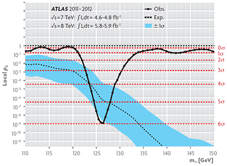
Figure 5. The solid curve (Obs.) represents the «observed» p-value for the null hypothesis (no signal) obtained from the variation of the likelihood in the fit of the invariant mass distribution of candidate events to Higgs bosons produced and decayed into two photons (Figure 3), two leptons and four leptons, with and without the signal component, based on the mass of the candidates (Aad et al., 2012). The dashed curve (Exp) indicates the «expected» p-value according to the predictions of the standard model, while the blue band corresponds to its uncertainty at 1s. In the region around the minimum observed p-value we can see that it (solid curve) is lower than the central value of the corresponding expected p-value (dashed curve) but consistent with the confidence interval at 1s (band). Since the p-value is smaller the higher the signal strength, we conclude that the data do not exclude that the signal is due to the Higgs boson of the standard model. The horizontal lines represent the corresponding p-values for statistical significance levels of 1 to 6s. The points on the solid line are the specific values of the boson mass used for the simulation of the signal with which the interpolation curve was obtained. / Source: ATLAS Experiment © 2014 CERN.

Another issue is to establish the true nature of the observation, starting with whether or not this is the Higgs boson of the standard model. Although the standard model does not predict its mass, it does predict, depending on this, its production cross-section and the probability that it will decay into a final state. This prediction is essential because, with the help of Monte Carlo simulations, it allows for the expected signal to be established with its uncertainty and the corresponding p-values in terms of mass, as shown in the dashed curve and the blue band in Figure 5. The comparison between the solid curve and the band indicates that the intensity of the observed signal is compatible with that expected at 1s (0.317 p-value, or equivalently, a probability content of 68.3 %), and thus the possibility that it is the Higgs boson of the standard model is not excluded. With the ratio between the two intensities we build a new statistical test that, when explored in terms of mass, provides the best estimate of the mass of the new particle and its confidence interval at 1s: 126.0 ± 0.4 ± 0.4 GeV, where the second (third) value denotes the (systematic) statistical uncertainty. Similar studies analysing the angular distribution of photons and leptons, a physical quantity sensitive to spin and parity (another quantum property with + and – values) of the boson, allowed to exclude p-values under 0.022 spin-parity assignments to 0–, 1+, 1–, 2+ versus the 0+ assignment predicted by the standard model (Aad et al., 2013; Chatrchyan et al., 2013).

With this information we cannot conclude, without risk of abusing statistical science, that we are faced with the Higgs boson of the standard model, but that it certainly resembles it.

References

Aad, G. et al., 2012. «Observation of a New Particle in the Search for the Standard Model Higgs Boson with the ATLAS Detector at the LHC». Physics Letters B, 716(1): 1-29. DOI: <10.1016/j.physletb.2012.08.020>.
Aad, G. et al., 2013. «Evidence for the Spin-0 Nature of the Higgs Boson Using ATLAS Data». Physics Letters B, 726(1-3): 120-144. DOI: <10.1016/j.physletb.2013.08.026>.
Aaij, R. et al., 2014. «Observation of the Resonant Character of the Z(4430)- State». Physical Review Letters, 112: 222002. DOI: <10.1103/PhysRevLett.112.222002>.
Agostinelli, S. et al., 2003. «Geant4-a Simulation Toolkit». Nuclear Instruments and Methods in Physics Research A, 506(3): 250-303. DOI: <10.1016/S0168-9002(03)01368-8>.
Arnison, G. et al., 1983. «Experimental Observation of Isolated Large Transverse Energy Electrons with Associated Missing Energy at √s=450 GeV». Physics Letters B, 122(1): 103-116. DOI: <10.1016/0370-2693(83)91177-2>.
Barlow, R. J., 1989. Statistics. A Guide to the Use of Statistical Methods in the Physical Sciences. John Wiley & Sons. Chichester (England).
Chatrchyan, S. et al., 2012. «Observation of a New Boson at a Mass of 125 GeV with the CMS Experiment at the LHC». Physics Letters B, 716(1): 30-61. DOI: <10.1016/j.physletb.2012.08.021>.
Chatrchyan, S. et al., 2013. «Study of the Mass and Spin-Parity of the Higgs Boson Candidate via Its Decays to Z Boson Pairs». Physical Review Letters, 110: 081803. DOI: <10.1103/PhysRevLett.110.081803>.
Cowan, G., 2013. «Statistics». In Olive, K. A. et al., 2014. «Review of Particle Physics». Chinese Physics C, 38(9): 090001. DOI: <10.1088/1674-1137/38/9/090001>.
Ellis, J., 2012. «Outstanding Questions: Physics Beyond the Standard Model». Philosophical Transactions of The Royal Society A, 370: 818-830. DOI: <10.1098/rsta.2011.0452>.
Feynman, R. P., 1963. The Feynman Lectures on Physics. Addison-Wesley. Reading, MA. Herb, S. W. et al., 1977. «Observation of a Dimuon Resonance at 9.5 GeV in 400-GeV Proton-Nucleus Collisions». Physical Review Letters, 39: 252-255. DOI: <10.1103/PhysRevLett.39.252>.
Nason, P. and P. Z. Skands, 2013. «Monte Carlo Event Generators». In Olive, K.A. et al., 2014. «Review of Particle Physics». Chinese Physics C, 38(9): 090001. DOI: <10.1088/1674-1137/38/9/090001>.
Nuzzo, R., 2014. «Statistical Errors». Nature, 506: 150-152. DOI: <10.1038/506150a>.
Physics Statistics Code Repository, 2002; 2003; 2005; 2007; 2011. PhyStat Conference 2002. Durham. Available at: <http://phystat.org>.
Schirber, M., 2013. «Focus: Nobel Prize-Why Particles Have Mass». Physics, 6: 111. DOI: <10.1103/Physics.6.111>.
Swanson, E., 2013. «Viewpoint: New Particle Hints at Four-Quark Matter». Physics, 6: 69. DOI: <10.1103/Physics.6.69>.
Webb, A., 2002. Statistical Pattern Recognition. John Wiley & Sons. Chichester (United Kingdom).