The map of biodiversity
From local to global scales
Species richness is not homogeneous in space and it normally presents differences when comparing among different sites. These differences often respond to gradients in one or several factors which create biodiversity patterns in space and are scale-dependent. At a local scale, diversity patterns depend on the habitat size (species-area relationship), the productivity, the environmental harshness, the frequency and intensity of disturbance, or the regional species pool. Regional diversity may be influenced by environmental heterogeneity (increasing dissimilarity), although it could act also at smaller or larger spatial scales, and the connectivity among habitats. Finally, at a global scale, diversity patterns are found with the latitude, the altitude or the depth, although these factors are surrogates for one or several environmental variables (productivity, area, isolation, or harshness).
Keywords: species richness, species-area relationship, productivity, latitudinal biodiversity gradient.
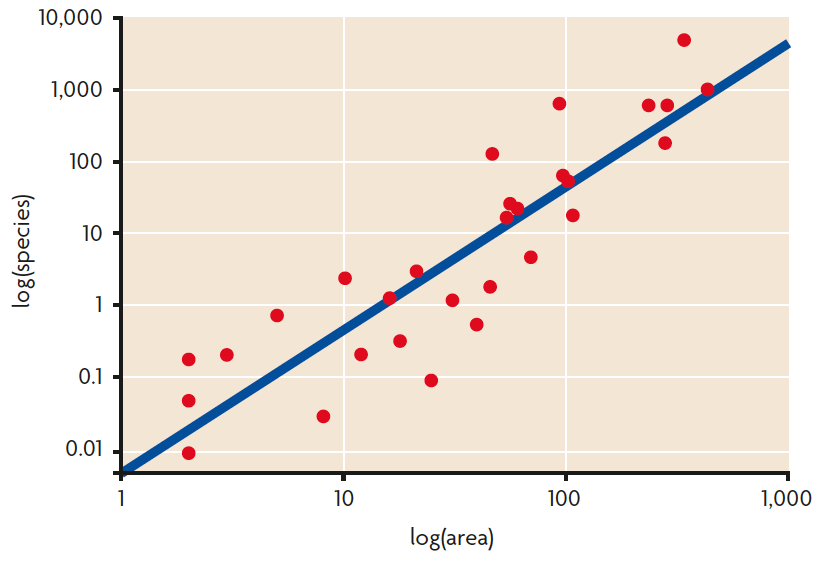
Figure 1. Species-area relationship (SAR) in the vascular plants of the Galapagos Archipelago: an increase in the sampled area results in an increase of the number of species found.
Why are some places more diverse than others?
A quick look at our nearby environment could serve to become aware that the distribution of species is not homogeneous in the space and that there are some sites that hold more species than others in comparable surface areas. Indeed, species present in a certain locality are the result of several processes occurring at different scales, such as geographical barriers, environmental constraints or biotic interactions that determine the assembly of ecological communities. All these processes define the composition of species in a given community: the number and identity of species (or biodiversity) in a certain area. Which specific factors influence this heterogeneous distribution of diversity in space? This question has driven the interest of naturalists since the time they started exploring the world. With the passing of time, they observed that biodiversity in many taxonomic groups followed predictable patterns in space, so that the spatial distribution of biodiversity could be explained by certain factors, and that the observed patterns were repeated across many regions around the globe.
«Naturalists observed that biodiversity in many taxonomic groups followed predictable patterns in space»
One of the first naturalists who reported the relationship between organisms and their environments was Alexander von Humboldt (1769-1859), who especially focused on the effect of geographical factors, such as climate, on different taxa. Humboldt’s work on the scientific expedition to America deeply inspired other naturalists to carry out their own explorations around the world, like Charles Darwin (1809-1882) or Alfred Russel Wallace (1823-1913). All these expeditions motivated the subsequent search for spatial patterns on species distributions and diversity at large scales. Since then, many different hypotheses have been proposed to answer this question, but the specific factors underlying diversity gradients are still controversial. Additionally, although some of the patterns can act at different scales, most of them are scale-dependent, so depending on the studied spatial scale, the factors related to the diversity gradients are not the same.
«Patterns of biodiversity at local scale were probably the first described, as a result of basic and simple observations in the field»
It is important to stress here that most studies analysing spatial patterns of biodiversity use the number of species (species richness) as the response variable. Recently, biologists have started to focus on different aspects of biodiversity such as the genetic or functional diversity. However, for simplicity, we will focus this review only on species diversity. Thus, we will use the terms biodiversity and species richness as synonymous hereafter. Below we will expand on biodiversity patterns across different spatial scales (summarised in Table 1).
Local patterns
Patterns of biodiversity at local scale were probably the first described, as a result of basic and simple observations in the field. One of the oldest patterns observed was the species-area relationship: the larger a sampled area is, the higher the number of species that will be found (Figure 1). This pattern has been observed worldwide, in terrestrial and marine environments. The first description of the species-area relationship dates back to the nineteenth century, when H. C. Watson noted, in a county of England, that the number of plant species sampled doubled for a 10-fold increase in the studied area (Connor & McCoy, 2000). Since then, the relationship has been firstly quantified by Arrhenius in 1921 with the power function S = cAz (where S is the number of species, A is the area, and c and z are constant parameters). The constants c and z are used to establish comparisons among different study areas.
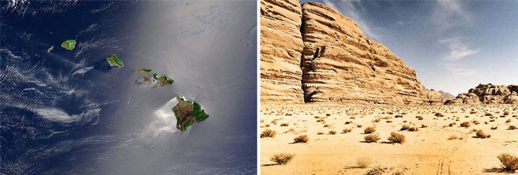
Figure 2. The species-area curves could be broken down in different patterns. One of them states that larger islands in an archipelago will harbor a greater number of species. This is one of the basis of the theory of island biogeography of MacArthur and Wilson. In the image, a satellite photo of the archipelago of Hawaii (USA). Figure 3. There are different factors that can shape biodiversity patterns; for example, environmental harshness as extreme temperatures. In the image, the desert valley known as Wadi Rum, in Jordan. /Jacques Descloitres, MODIS Land Rapid Respon-se Team, NASA GSFC / Martino Pietropoli
Rosenzweig (1997) considered that the species-area curves could be actually broken down in four different patterns. The two first ones depend on the size of the sampled areas: small and large. A third one considers the macroscale (biogeographical provinces), so the increase of species is not related with immigration of species from other areas, but with speciation processes, which act in a slower temporal scale. And the fourth pattern is one of the basis of the theory of island biogeography of MacArthur and Wilson, which states that larger islands in an archipelago will harbor a greater number of species (Figure 2). Two main arguments are used to explain species-area relationship: first, larger areas can sustain larger populations and thus, the species have a lower probability of going extinct; and second, larger surface areas have higher habitat heterogeneity (explained below at regional scale).
| Scale | Factor |
| Local | Area |
| Ecosystem productivity | |
| Environmental harshness | |
| Disturbance level | |
| Regional species pool | |
| Regional | Environmental heterogeneity |
| Connectivity | |
| Global | Latitude |
| Altitude (in mountains) | |
| Depth (in marine ecosystems) |
Table 1. Summary of the different factors creating spatial diversity patterns and the scales at which mainly operate: local, regional, and global. In some cases, the factor is not the underlying cause for the diversity gradient, but a sum of different variables is creating the pattern (e.g., latitude; see text).
Other widely studied pattern is the relationship between species richness and ecosystem productivity. Productivity is the rate at which biomass is produced in a given area, so it is a measure of the energy input in the ecosystem (normally estimated through precipitation, evapotranspiration, or nutrient supply). It was originally thought that resources tend to be unlimited at higher productivity levels, allowing the presence of a greater number of species. This pattern is mainly observed at global scales, where biogeographic regions with a higher energy input generally hold more species (see the global scale section). At local scales, different kinds of relationships have been observed: positive, negative, U-shaped and hump-shaped (Mittelbach et al., 2001). The latter is found when biodiversity is higher at intermediate levels of productivity, and it is frequent enough in nature to have spurred several studies trying to explain its underlying causes. In the first part of the productivity gradient (low to intermediate productivity), there is an increase in species diversity following an increase in resources availability. However, the decrease in species richness after a certain productivity level (“the paradox of enrichment”) is less clear. Different hypotheses have been suggested, such as the increase in competitive exclusion at high productivity levels or the shift in the limiting resource from nutrients to light for plants (Tilman & Pacala, 1993). Yet not a single hypothesis explains the variation in the shape and strength of the relationship between productivity and diversity, and factors such as the spatial scale, the studied taxa, the type of habitat (terrestrial or aquatic) or the intensity of predation (exploiter-mediated coexistence) may be relevant to explain these disparities.
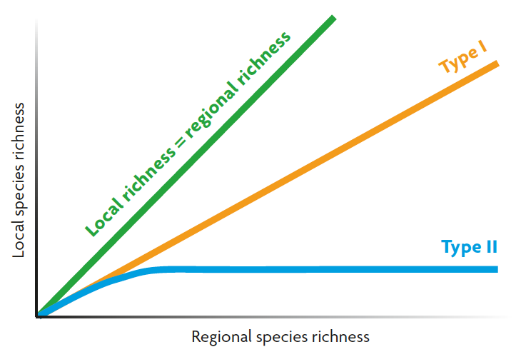
Figure 4. Relationship between local and regional species richness, showing the theoretical line, when local richness equals regional richness, and the two different types of response: Type I, a positive relationship when the composition of local patches depends on the regional richness, and Type II, when local patches have specific characteristics that impede the entrance of species from the regional species pool.
While both area and productivity favor the coexistence of numerous species, other factors shape biodiversity patterns by limiting their numbers. For example, environmental harshness (e.g., acidic and highly alkaline habitats, extreme temperature) selects species that can persist in these habitats, organisms that present very specific adaptations (Figure 3). However, to complicate matters further, these habitats may also share some common features that might contribute to the low species richness, such as small area or isolation (for example hot springs or mountain peaks), making it difficult to disentangle the effect of these multiple factors on local diversity. Another hypothesis proposed to explain diversity gradients is the intermediary disturbance hypothesis (Connell, 1978), which proposed that habitats with high and low disturbance levels contain few species. Thus, maximum diversity should be found at intermediate levels of disturbance (Connell, 1978), because it should preclude the dominance of good colonisers (at high disturbance levels) and good competitors (at low levels). Although it was firstly demonstrated empirically in intertidal boulders with different degrees of storm intensity (Sousa, 1979), studies in other systems have not been able to find evidence supporting the intermediary disturbance hypothesis.
«One of the main factors creating a diversity gradient at a regional scale is the environmental heterogeneity»
Finally, the size of the regional species pool is relevant for the local diversity. What would happen in local communities where we have a gradient in regional species richness? Theoretically, two different responses could be observed (Figure 4). The first one is found when the composition of local communities depends greatly on the regional species pool (species that arrive and colonise the local communities). In this case, a linear positive relationship will be found: as the regional diversity increase, the local diversity will do so (type I curve). The second one will be expected when local communities present some features (e.g., competition or predation) that limit the indiscriminate entrance of species from the species pool. In this case, the local richness will saturate with regional richness because the number of ecological spaces at the local habitats are limited (type II curve). Empirical studies have concluded that type I response is the most common in nature.
Regional patterns
A region is considered to include a large number of habitats and communities, and it is often referred as the area from which species may colonise local communities. Thus, one of the main factors creating a diversity gradient at a regional scale is the environmental heterogeneity: if the environment in the region is homogeneous, its communities will likely contain the same species, which in turn will result in a low regional species richness.1 On the contrary, a broad variation in environmental conditions across different habitats in a region will allow the presence of diverse communities (high dissimilarity)2 and high regional species richness (Figure 5). The positive relationship between environmental heterogeneity and species richness has been proven empirically across taxa, ecosystems and at different spatial scales (Stein, Gerstner, & Kreft, 2014). Thus, in addition to the variety of habitats in a region, this pattern also operates at smaller (microhabitat heterogeneity at local scales) and larger spatial scales (habitat gradients at a global scale).
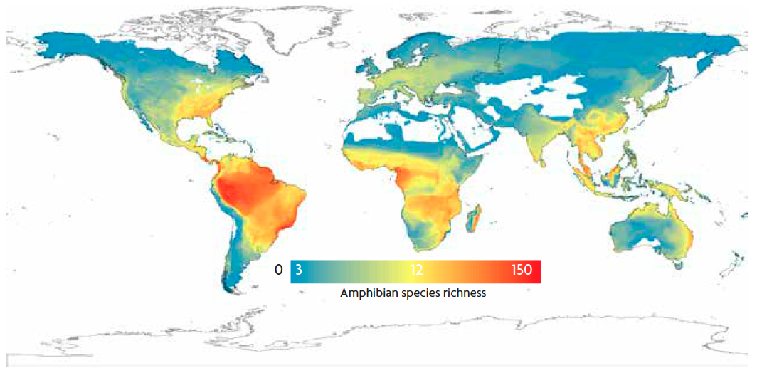
Figure 6. Latitudinal diversity gradient in amphibians, including 6,117 species in 5o grid cells. The number of species is higher in the tropics and decreases gradually towards the poles. The colour gradient indicates a variation from 3 species per cell (blue), to 12 (yellow), and 150 (red) approximately. / Pyron & Wiens, 2013. Published by the Royal Society. All rights reserved.
In the last decades, with the increasing interest on metacommunities (a set of local communities linked through dispersal), the flow of individuals among local patches has been taken into consideration. One of the important factors influencing this flow is the degree of connectivity of local patches, determined by the location of each patch in the landscape (Borthagaray, Pinelli, Berazategui, Rodríguez-Tricot, & Arim, 2015). Then, depending on the configuration of the metacommunity network, as well as the dispersal capabilities of the species and their body-size, the local and the regional species richness would vary. For example, in the case of organisms with low dispersal rates, when patches are isolated, local diversity would be low, but regional would be high. On the contrary, when organisms disperse at high rates and patches have a high connectivity, local diversity would be high, but regional diversity low.

Figure 7. Illustration of the «mid-domain effect» using pencils as one of the possible explanations of the latitudinal diversity gradient (decrease of diversity from the equator to the poles, or any other clearly demarcated area): randomly, the center parts of a box full of pencils of different sizes will contain more pencils (or parts of them) than the outer areas. / Community Ecology
Global patterns
The first evidences of biodiversity gradients at large scales emerged from the first European expeditions to the New World after the eighteenth century. In these explorations, naturalists were sent to describe the exotic species found there and get new insights about the mysterious and exotic nature of this new continent. Many of them were fascinated by the great diversity of species (and their shapes, colours and behaviour) that were found in the tropics in comparison with the well-known European regions. These observations have led to the description of the most famous large-scale biodiversity pattern: the latitudinal diversity gradient, which is characterised by a decrease in species richness from the equator to higher (north or south) latitudes (Figure 6). This decay in diversity is slightly asymmetrical between the Northern and the Southern Hemisphere, with a steeper slope in the Northern Hemisphere. The latitudinal diversity gradient has been documented for a variety of animal and plant taxa across different ecosystems (marine and terrestrial; Hillebrand, 2004). Nonetheless, some exceptions exist. For instance, aquatic macrophytes represent one of the few taxonomic groups that show a reverse latitudinal diversity gradient, as richer communities are found at higher latitudes.
Additionally, this gradient is not only observed on present-day species, but also on the fossil record (it has been mainly observed in some invertebrate marine taxa, such as Brachiopoda or Foraminifera). However, latitude itself is not the underlying cause of this biodiversity gradient. Instead many environmental factors that could explain this gradient correlate with latitude. Until now, many different mechanisms have been suggested, and probably a combination of some of them will be influencing the diversity variation across the latitudinal gradient. Mittelbach (2012) summarises all the different hypotheses in four: ecological, historical, evolutionary hypotheses, and null model. The ecological hypotheses are mainly based in the relationship between productivity (such as energy input and resource availability) and a higher abundance of individuals, which will reduce the probability of extinction. The historical hypotheses defend that the tropics are older, with a greater geographic extent (in the past and nowadays) and with more stable climatic conditions across periods, so they have had more time for diversification. The evolutionary hypotheses focus on the higher rates of diversification in the tropics. And finally, the null model is based in the «mid-domain effect»: the idea that if the distribution ranges of species are randomly placed along the latitudinal gradient, it is more probable that a higher number of species distributions will overlap in the middle (the equator). This can be easily visualised with a box full of pencils of different sizes, so just by chance, most parts of the pencils will be in the center of the box (Figure 7).
«The latitudinal diversity gradient is not only observed on present-day species, but also on the fossil record»
While the latitudinal diversity gradient is the most enthralling pattern in ecology, other global patterns have been described, such as elevation gradients in mountain systems and depth gradients in marine environments. Like latitude, these two variables are not causal factors underlying species richness patterns. In these cases, the increasingly harsh environmental conditions along the altitude and depth gradients, as well as the low productivity, isolation or reduced surface areas (e.g., highest peaks) may contribute to the decrease in species richness.
What can we learn from spatial patterns in biodiversity?
We have presented here the most studied biodiversity patterns at different spatial scales. Some of them present a generalised and clear relationship with diversity, while in other cases the response is questionable and needs further investigation. However, we stress that most of these patterns are established with a huge amount of ignorance regarding species taxonomy and distribution, especially at the global scale (the Linnean and Wallacean shortfalls, respectively; Hortal et al., 2015). These knowledge gaps reflect not only the differences in survey effort worldwide, but also the inequality in the studied taxa. For instance, datasets are much more complete for vertebrates (birds or mammals) and some groups of plants (trees) than for invertebrates and other small taxa. Likewise, aquatic habitats are less studied despite their disproportionally high contribution to global diversity, and there is still some uncertainty whether biodiversity in aquatic environments follows the same patterns as in terrestrial habitats (Siqueira, Bini, Thomaz, & Fontaneto, 2015). Filling these gaps will help elucidating the ubiquity of the spatial patterns and the exceptions (if any) to them.
«The first evidences of biodiversity gradients at large scales emerged from the first European expeditions to the New World after the eighteenth century»
The relevance of spatial biodiversity gradients and the drivers that cause them is not only important from a naturalistic point of view, but it has relevant implications for biodiversity conservation. For example, hotspots of diversity worldwide may be established following these gradients. At global scale, the importance of the tropics for biodiversity is unquestionable, so major conservation efforts should be focused on these areas. At local and regional scales, protected areas should be designed considering the environmental factors that maximise the preservation of biodiversity. Thus, factors as the delimitation of the size, the inclusion of different habitats to increase heterogeneity, or the connectivity and isolation of patches should be considered. Finally, after experimental and fieldwork in the last decades of the twentieth century, nowadays the benefits that biodiversity provide are well recognised. In addition to invaluable goods (food, water, or medicines), biodiversity is correlated with ecosystem functioning and services: it enhances productivity, nutrient cycling, ecosystem stability, or resistance to invasive species. Thus, knowing and preserving the areas with high diversity will contribute to maintain these benefits.
1. The number of species found in a region is known as gamma diversity. (Go back)
2. The dissimilarity and similarity between local communities is known as beta diversity, which is a measure of the difference in species composition between two or more habitats within a region. (Go back)
References
Borthagaray, A. I., Pinelli, V., Berazategui, M., Rodríguez-Tricot, L., & Arim, M. (2015). Effects of metacommunity networks on local community structures: From theoretical predictions to empirical evaluations. In A. Belgrano, G. Woodward, & U. Jacob (Eds.), Aquatic functional biodiversity: An eco-evolutionary approach (pp. 75–111). London/San Diego, CA/Waltham, MA/Oxford: Academic Press (Elsevier).
Connell, J. H. (1978). Diversity in tropical rain forests and coral reefs. Science, 199, 1302–1310. doi: 10.1126/science.199.4335.1302
Connor, E. F., & McCoy, E. D. (2000). Species-area relationships. In S. A. Levin (Ed.), Encyclopedia of biodiversity (pp. 397–411). New York, NY: Elsevier. doi: 10.1016/B0-12-226865-2/00252-2
Hillebrand, H. (2004). On the generality of the latitudinal diversity gradient. The American Naturalist, 163(2), 192–211. doi: 10.1086/381004
Hortal, J., De Bello, F., Diniz-Filho, J. A. F., Lewinsohn, T. M., Lobo, J. M., & Ladle, R. J. (2015). Seven shortfalls that beset large-scale knowledge of biodiversity. Annual Review of Ecology, Evolution, and Systematics, 46, 523–549. doi: 10.1146/annurev-ecolsys-112414-054400
Mittelbach, G. G. (2012). Community ecology. Sunderland, MA: Sinauer Associates.
Mittelbach, G. G., Steiner, C. F., Scheiner, S. M., Gross, K. L., Reynolds, H. L., Waide, R. B., … Gough, L. (2001). What is the observed relationship between species richness and productivity? Ecology, 82(9), 2381–2239. doi: 10.2307/2679922
Rosenzweig, M. L. (1997). Species diversity in space and time. Cambridge: Cambridge University Press.
Siqueira, T., Bini, L. M., Thomaz, S. M., & Fontaneto, D. (2015). Biodiversity analyses: Are aquatic ecologists doing any better and differently than terrestrial ecologists? Hydrobiologia, 750, 5–12. doi: 10.1007/s10750-014-2071-6
Sousa, W. P. (1979). Disturbance in marine intertidal boulder fields: The non-equilibrium maintenance of species diversity. Ecology, 60, 1225–1239. doi: 10.2307/1936969
Stein, A., Gerstner, K., & Kreft, H. (2014). Environmental heterogeneity as a universal driver of species richness across taxa, biomes and spatial scales. Ecology Letters, 17(7), 866–880. doi: 10.1111/ele.12277
Tilman, D., & Pacala, S. (1993). The maintenance of species richness in plant communities. In R. E. Ricklefs & D. Schluter (Eds.), Species diversity in ecological communities (pp. 13–25). Chicago: The University of Chicago Press.
This work was carried out with the support of CAPES (Coordenação de Aperfeiçoamento de Pessoal de Nível Superior), of the Brazilian Ministry of Education.