Old mathematical challenges

The Millennium Problems set out by the Clay Mathematics Institute became a stimulus for mathematical research. The aim of this article is to highlight some previous challenges that were also a stimulus to finding proof for some interesting results. With this pretext, we present three moments in the history of mathematics that were important for the development of new lines of research. We briefly analyse the Tartaglia challenge, which brought about the discovery of a formula for third degree equations; Johan Bernoulli’s problem of the curve of fastest descent, which originated the calculus of variations; and the incidence of the problems posed by David Hilbert in 1900, focusing on the first problem in the list: the continuum hypothesis.
Keywords: cubic equation, Cardano–Tartaglia formula, brachistochrone, Hilbert’s problems, continuum hypothesis.
The Clay Mathematics Institute has chosen seven mathematical problems and is offering a million dollars to anyone who can solve one of them. Mathematical challenges are not unprecedented, and so in this text, we present several preceding historical challenges. We have excluded controversies such as those between Newton and Leibniz, D’Alembert and Bernoulli, or Cantor and Kronecker and also leave aside the prizes offered by the academies of science (such as those offered by the French or the Prussian academies since the eighteenth century).
Hence, we will show several aspects of the development of mathematics from a special perspective. Carl Benjamin Boyer (1989) and Morris Kline (1972) are key references in the history of mathematics, but another more informative book is that of William Dunham (1990). In addition, the website of the University of St. Andrews (Scotland) is also a very valuable source of historical material (mainly biographies).
Tartaglia’s challenge
Ancient Mesopotamian mathematicians had already formulated a number of instructions (with no explanation) to find specific solutions to problems that could be described today with quadratic equations. Speaking in modern terms, if the unknown verifies the equation x2 + px + q = 0, then the solution is given by
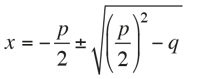
In the spirit of honesty, here we have not only used modern notation, but we have also taken some liberties with the language, because in ancient times p and q were always positive amounts and positive solutions were sought.
In principle, the equation could be associated with the calculation of an area, thus the use of the square. Therefore, it makes sense to consider cubic equations associated with the calculation of volumes. Indeed, the cubic equation was posed, and even solved, geometrically. Such a result arrived thanks to the Persian mathematician Omar Khayyam (1048-1131), who used conic sections (that is to say, ellipses, parabolae, and hyperbolae) whose intersections provided the roots. On the other hand, with patience, the roots of any polynomial can always be approximated. For instance, Leonardo of Pisa (ca. 1170-1250), also known as Fibonacci, expressed the approximation to the root of a cubic equation. The fact is that, at the end of the Medieval era, there were already methods for calculating the roots of cubic equations geometrically or approximately. However, the expression for obtaining them was not known at the time and, according to the influential Luca Pacioli (1445-1517), finding the formula to a general cubic equation was as difficult as squaring the circle.
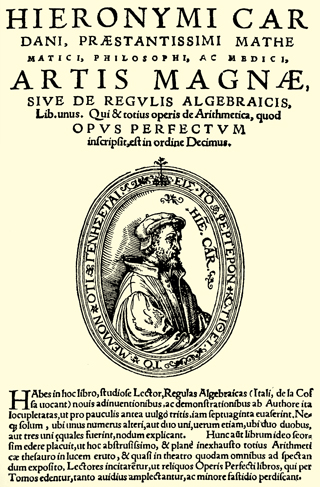
Niccolò Fontana, nicknamed Tartaglia, told Girolamo Cardano how to solve cubic equations, under the promise of keeping it a secret. But Cardano did not comply and published the formula in the book Ars Magna in 1545. / Mètode
The argument around the cubic equation arrived in 1535. Challenges and betting were common at the time. One of the protagonists of the discussion was Niccolò Fontana (1500-1557), nicknamed Tartaglia (“the stammerer”). He arrived in Venice in 1534 and acquired fame as a good mathematician. Apparently, he said he could solve some specific instances of cubic equations and so, Antonio Maria del Fiore challenged Tartaglia. Each opponent proposed a list of thirty problems to be solved within a fixed span of time. The one who solved fewer problems would pay for dinner for the other and as many of their friends as problems the winner had solved. The point is that Del Fiore knew a formula to solve a type of cubic equation, revealed to him by Scipione del Ferro (1465-1526) shortly before his death. Therefore, all the problems proposed to Tartaglia were incomplete cubic equations. Tartaglia understood that Del Fiore had a formula, and so he searched for it until he finally discovered it. The day the result was to be decided, Tartaglia had solved all the problems proposed by Del Fiore, while the latter had been unable to solve any of Tartaglia’s.
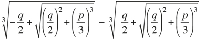
In current terms, the cubic equation studied by Tartaglia was x3 + px + q = 0, although he always wrote words instead of the p and q coefficients. The solution is provided by the Cardano–Tartaglia formula. According to it, x equals::
After the dispute, it became obvious to everyone that Tartaglia had a formula for cubic equations, but he did not publish it. Girolamo Cardano (1501-1576) then started pressuring Tartaglia to tell him how to solve cubic equations. Finally, Tartaglia told him the rule, in code, but under the promise to keep it secret. However, Cardano did not comply and he published the formula in the book Ars Magna in 1545. In addition to Tartaglia’s solution, the rule for solving the general equation x3 + nx2 + pq + q = 0, obtained by Cardano in collaboration with his disciple Ludovico Ferrari (1522-1565), can also be found in the book. The fact that the book contained the solution to a general quartic equation was even more surprising; Ferrari had discovered it using similar techniques to the ones he had used when learning to solve cubic equations.
«After the efforts of many mathematicians over more than two centuries, Niels Abel proved the impossibility of solving a general equation of degree higher than four in radicals»
All this work was the starting point for two lines of mathematical research. On the one hand, the search for a formula to solve quintic equations had started. After the efforts of many mathematicians over more than two centuries, including that of important figures such as Joseph-Louis Lagrange (1736-1813), the Norwegian Niels Abel (1802-1829) proved the impossibility of solving a general equation of degree higher than four through radicals. However, the story did not end there because the rules for when the solution to a quartic equation could be found through radicals still remained unknown. Shortly before dying in a duel, Évariste Galois (1811-1832) wrote a document in which he proved a theory to determine whether or not a polynomial equation was solvable via radicals. The publication of Galois’s document in 1846 can be considered the starting point of modern algebra.
«The publication of a document by Évariste Galois in 1846 can be considered the starting point of modern algebra»
On the other hand, there was an important case in the formula of cubic equation that occurs when (q/2)2 + (p/3)3 < 0. Cardano and Ferrari called this «casus irreducibilis». The fact that cubic equations always have roots is well known. What happens when we also apply the formula in this case? Simply, we find expressions involving the cubic and square roots of negative numbers. For example, let us assume that we already know that one root of x3 − 15x − 4 = 0 és x = 4, but if we try to apply the rule, we obtain:

Using formal substitutions, we can deduce that:
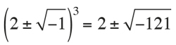
and, consequently, we arrive to:
![]()
![]()
The issue this calculation illustrates is the fact that using the square roots of negative numbers can be useful. It is the origin of complex numbers. Likewise, Cardano and Ferrari realised that, using these strange numbers, every cubic equation has three roots and every quartic equation has four. It is the first version of the so-called «fundamental theorem of algebra»: every n degree polynomial has exactly n complex roots (taking into account repeated roots). Later, complex number research would lead to the theory of functions of a complex variable, whose properties are very different from the functions of a real variable (for example, every differentiable function in a disk can be represented by a power series).
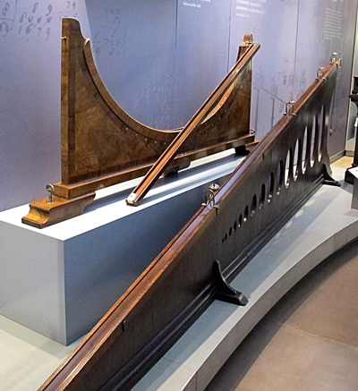
We could say that the curve of fastest descent is the one that allows for the optimal design of a slide. Dropping balls on an inclined plane and a circumference, Galileo Galilei realised that the descent was faster on the latter. In the picture, a device created by Francesco Spighi to compare the speed of a ball falling on a cycloid and a straight line. It can be found on the Galileo Museum in Florence. / Sailko/Wikimedia
The curve of fastest descent
One of the forerunners of differential calculus, Pierre de Fermat (1601-1665), discovered a method for calculating maximums and minimums: today we say that if point x is a maximum or a minimum for a particular smooth function f, then f’(x) = 0. He applied this method to the study of light rays, together with the principle that states that light travelling between two points takes the path requiring the shortest time. Thanks to that, he deduced the law of reflection and refraction (Snell’s law); the latter assumes that light moves more slowly in a denser medium. The fact that Snell’s law was later used by Johann Bernoulli (1667-1748) is significant; he considered a non-homogeneous optical medium comprising parallel layers of variable density that overlap horizontally in order to find the curve of fastest descent. The idea was that light in this medium would travel along precisely the curve he was looking for, which he called «brachistochrone».
What is the curve of fastest descent? The formal definition is as follows: given two points, A and B, in a vertical plane, where A is higher than B, the curve of fastest descent is the one followed by a given weight when it travels from A to B in the shortest possible time under the influence of gravity. In other words, the curve of fastest descent is the one that allows for the optimal design of a slide. Usually, the first thing that comes to mind would be straight line, since that is the shortest curve between two points. But Galileo Galilei (1564-1642) realized that was not the case. Dropping balls on an inclined plane and on a circumference, he observed that the descent was faster on the circumference.
To understand this properly, let us consider point A = (0,0) and B = (1,–1). where we want to discover which of all the y = f(x) functions that satisfy f(0) = 0 and f(1) = –1, has the fastest falling time for a given weight (T) following the graph of the function. Reasoning using the laws of physics brings us to the amount that must be minimised:
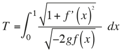
were g stands for the gravity constant. Now, following Galileo, we can calculate the time taken on different curves. For the straight line f(x) = –x, we obtain
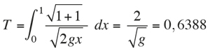
and for the circumference arc

we obtain
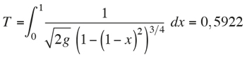
In other words, Galileo was right. However, the circumference is not the brachistochrone either. The shortest time is reached when T = 0,5832.
In the June 1696 issue of the German journal Acta Eruditorum, Johann Bernoulli proposed the challenge of finding the brachistochrone to the mathematics community. He claimed that he had the answer and that it was a curve that is very well known to geometers. In May 1697, Bernoulli published that four mathematicians had managed to prove that the brachistochrone was the cycloid; that is, the curve defined by a point of the circumference as it rolls along a straight line without slipping (for instance, a point on a car’s tyre in contact with the pavement). These mathematicians were Gottfried Wilhelm Leibniz, Jakob Bernoulli, the Marquis de L’Hôpital Guillaume François Antoine, and an anonymous mathematician, and each one proved it in a different way.
The formal challenge seemed to be an invitation especially directed toward Isaac Newton (1643-1727), so it would not have been surprising if he had answered it. Legend says that Newton received the problem after a tiring working day at the mint and he focused on it for twelve hours until he solved it: it was the problem that cost Newton a whole night. He answered anonymously, but Bernoulli guessed the author when he saw it and claimed he knew it was Newton’s work, just as «we know the lion by his claw».
The brachistochrone problem was one of the first examples of what later became the calculus of variations. The goal is to minimise a quantity, time in this case, which does not depend on a finite number of independent variables, but on the global shape of the curve. A typical problem in the calculus of variations is the finding of the function that minimises an integral such as
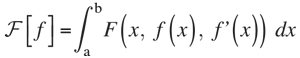
for a given function F(x, y, y’). One might try to apply Fermat’s idea: to (somehow) derive the «function» F and make F’[f] = 0 in order to obtain a condition of the function f. The studies by Leonhard Euler (1707-1783) and Joseph-Louis Lagrange (1736-1813) discovered that these procedures led to the following condition:
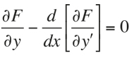
The reasoning, however, was not rigorous, and we had to wait until the nineteenth century before a satisfactory basis for the calculus of variations was provided by Karl Weierstrass (1815-1897) and David Hilbert (1862-1943).
Meanwhile, mathematicians had proposed problems requiring the minimisation of multiple integrals, such as those in potential theory, which try to minimise the integral
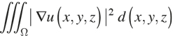
between all the functions u using continuous partial derivatives in order to verify a condition at the boundary of Ω. On the other hand, physicists had already applied ideas from the calculus of variations to mechanics, leading to the emergence of analytical mechanics with both the Lagrangian and the Hamiltonian formulation. The generalisation of Fermat’s idea underlay this: nature economises all of its actions and consequently, all natural phenomena have one (or more) quantity that must be minimised.
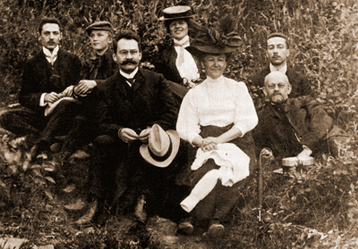
In 1900, the mathematician David Hilbert proposed a list of twenty-three unsolved problems from every field in mathematics, to serve as examples of questions that would be fundamental in the starting century. The photo shows Hilbert – front row, on the right – with some friends. / Yeshiva University
Hilbert’s twenty-three problems
In the summer of 1900, David Hilbert was almost at the peak of his career. His résumé included the solution to Gordon’s problem about the invariants in certain algebraic forms, as well as the impulse he has given to algebraic number theory, the axiomatisation of geometry, and the justification of Dirichlet’s principle under certain hypotheses. He was one of the most renowned mathematicians of the time when he delivered a lecture at the Second International Congress of Mathematicians in Paris.
His lecture, «Mathematical problems» (which can be found in Hilbert, 1902) manifested his absolutely optimistic mathematical philosophy. In addition, he proposed a list of twenty-three unsolved problems from every field of mathematics, as examples of questions whose resolution he believed would be fundamental in the coming century. The list focused the efforts of many mathematicians and became very influential (without question, because of Hilbert’s authority). In short, anyone who solved one of these problems acquired a solid reputation.
«A considerable part of the mathematical development during the twentieth century stemmed from Hilbert’s list»
lbert’s research lines exactly. Even he could not have guessed the new fields that would soon appear, in some cases, such as spectral theory, with the help of Hilbert himself. However, a considerable part of the mathematical development during the twentieth century stemmed from Hilbert’s list. In the following section we briefly introduce the first problem on the list.
Continuum hypothesis
At the end of the nineteenth century, Georg Cantor (1845-1918) systematically analysed infinity. In his theory, two (finite or infinite) sets have the same cardinal if a bijection exists between them. Note that, when the set is finite, its cardinal is the number of elements it contains.
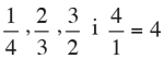
Applying his definition to the set of all positive integers, N, and to the set of all rational numbers Q (those that can be written as m/n, where m and n are integers, and n ≠ 0), he proved that they both had the same cardinal. This is the smallest infinite cardinal, and is denoted ℵ0. When ℵ0 is the cardinal of a set, since a bijection between it and the set of positive integers exists, the elements in the set can be written as a sequence. It is not too difficult to understand the proof that the cardinal of Q is ℵ0 when one knows the procedure. We consider m/n a rational number written as an irreducible fraction where m and n are positive and the sum m + n is a fixed amount. If m + n = 2, then:

If m + n = 3, then:
![]()
If m + n = 4, then:

If m + n = 5, then:
Evidently, continuing the process for m + n = 6, 7, etc. we will include all the positive rational numbers.
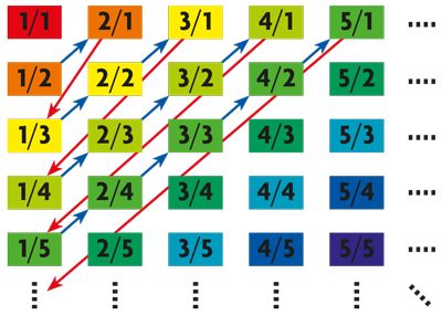
Process for expressing positive rational numbers as a sequence. / Sergio Segura
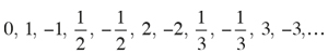
We must also include 0 and the negative numbers, and so we alternate them with the positives. The first elements in the sequence that contains all the rational numbers are:
Later, Cantor proved that the set of all polynomial roots with integer coefficients has the same cardinal.
The issue changed when it was discovered that the set R of real numbers (those that can be written with decimals even if they are irrational) is larger than ℵ0, which was demonstrated by reductio ad absurdum. Cantor assumed that all the numbers between 0 and 1 could be written in a sequence, and found a number that did not belong in that sequence. This might be the first significant theorem in his theory, and it shows that there are different types of infinity. The fact that most real numbers are irrational is a consequence of this. Moreover, most real numbers are not the root of any polynomial with integer coefficients. The result was very surprising at the time, taking into account that few numbers of this type were known.
Looking closer at his analysis, he proved that there are as many real numbers as there are subsets of N. However, he did not find any set with a cardinal higher than ℵ0 and lower than that of R. Thus, he conjectured that the cardinal of R was the second infinite cardinal; this is the continuum hypothesis, which states that any infinite subset of the set of real numbers can be bijected with the set of natural numbers or the set of real numbers.
In the following years, a lot of effort was put into trying to prove Cantor’s conjecture. They were all unsuccessful, and Hilbert posed the problem as the first on his list. The solution took time, and is not easy to understand.
The first step was taken by Kurt Gödel (1906-1978). In 1940, he proved that if the usual axiomatic system of set theory is consistent, so is the continuum hypothesis added to the system. In other words, the continuum hypothesis does not contradict the other axioms considered in set theory. Therefore, a set with a cardinal higher than ℵ0 and lower than the cardinal of R cannot be discovered, since it would be a contradiction. But this does not prove the continuum hypothesis.
We owe the second step to Paul Joseph Cohen (1934-2007), who in 1963 proved that the continuum hypothesis is in fact different from the other axioms. Indeed, using a method he called «forcing», he observed that if the axiomatic system of set theory is consistent, then it would remain consistent when the rejection of the continuum hypothesis was incorporated into the system. The conclusion is that neither the continuum hypothesis nor its rejection can be proved with the usual axiomatic system of the set theory. We can add another axiom stating that the continuum hypothesis is true (or add a different one claiming it is false). With current axioms, our ignorance of the matter is absolute.
According to Gödel, that was not the end of the problem. What we have seen is that the axioms of set theory are insufficient to answer the question and they must be complemented with others. In the future, mathematicians will add new axioms to the system. The criteria for adding them will be that they have desirable consequences (according to our mathematical intuition) and will not have undesirable consequences. Gödel thought that Cantor’s conjecture was false. With the new axioms, we will be able to formulate the problem of the continuum hypothesis again.
Beyond Hilbert’s problems
Hilbert’s conference had so many repercussions that, in order to commemorate it, the International Mathematical Union declared the year 2000 the World Mathematical Year and asked prestigious mathematicians for lists of problems. Stephen Smale, for example, proposed eighteen. But no list has received as much attention as the Clay Mathematics Institute prize, announced in May 24, 2000. As it happened with Hilbert’s list, it contains problems from all the great fields of mathematics. Only one, the Poincaré conjecture, has been solved. In the following articles in this monograph, you can find brief introductions to these problems: I invite you to take a look for yourselves.
References
Boyer, C. B. (1989). A history of mathematics. New York: John Wiley & Sons, Inc.
Dunham, W. (1990). Journey through genius. New York: John Wiley & Sons, Inc.
Hilbert, D. (1902). Mathematical problems. Bulletin of the American Mathematical Society, 8, 437–479. doi: 10.1090/S0002-9904-1902-00923-3
Kline, M. (1972). Mathematical thought from ancient to modern times. New York: Oxford University Press.