Navier-Stokes equations

Mathematically, the motion of a fluid is described by the so-called Navier-Stokes equations. In the spirit of Newtonian mechanics, these equations should determine the future motion of the fluid out of its initial state. However, despite the significant effort made for more than a century, this determinism has not yet been mathematically proved nor disproved. This paper offers a general perspective on the Navier-Stokes equations, the fourth millennium problem.

Keywords: Navier-Stokes equations, fluid mechanics, meteorology, Newtonian determinism, millennium problems.

Hurricane Matthew pummelled across the Caribbean Sea between 28 September and 10 October 2016, but the phenomenon was not predicted until four days before, and even then it was only assigned a 70% probability. In the picture, the hurricane on 4 October 2016. / NASA Earth Observatory / Joshua Stevens

A practical-interest problem

One of the most treasured values of science is its ability to predict events. Celestial mechanics is particularly remarkable, since it allows us to predict, for instance, that on 14 May 2887 an annular solar eclipse will be visible from my city immediately after sunrise.

In meteorology, where there is a lot of practical interest in forecasts, the situation is quite different. Despite the remarkable advances that have been made in this field, predictions still cannot be made far enough in advance, even about very intense and widespread phenomena. Thus, hurricane Matthew pummelled across the Caribbean Sea between 28 September and 10 October 2016, but the phenomenon was not predicted until four days before, and even then it was only assigned a 70% probability.

Further, it does not look like data resolution or calculation-power are to blame for this. These parameters are constantly improved, but this does not significantly affect the timeliness of meteorological forecasts. Therefore, it is natural to wonder if there might be an intrinsic limit on how long in advance predictions can be made in this field.

«One of the most treasured values of science is its ability to predict events»

It is not only about the famous «butterfly effect», which results from the limited precision of the data. What we are putting forward is the possibility that the future might be unpredictable even if the data were infinitely precise!

It can be argued that meteorological processes are very complex. In view of this, it is advisable to bypass non-essential complications and consider a simpler system – the simpler the better – where the question we are posing continues to make sense: whether or not there is an intrinsic limit to the time extent of predictions.

«It is natural to wonder if there might be an intrinsic limit on how long in advance predictions can be made in this field»

Let us consider, for instance, a closed and immobile container completely filled with water. Let us assume that just before closing the container, we set the water in motion with some strength. Let us assume also that, just after closing the container, we knew exactly the magnitude and direction of the water velocity at each point. Would it then be possible to predict the values of these same variables for any time in the future until the water becomes practically at rest?

Despite previous significant advances, meteorological predictions still cannot be made far enough in advance, even about very intense and widespread phenomena. Above, an anticyclonic tornado in Simla, Colorado (USA) in June 2015. / James Stuart

The equations of motion

The possibility of predicting the future in a mechanical system is based on the so-called equations of motion. In the case of celestial mechanics, we are talking about Newton’s second law combined with the law of universal gravitation. According to these laws, celestial bodies cannot move however they want to. The acceleration of each body – the second time-derivative of its position – is determined by the position of all the other bodies in relation to it. As Newton showed, this allows to calculate how the velocities and positions of each body will be changing, as long as we know the initial values of these same variables.

The extension of these ideas to the case of a fluid is not trivial. To begin with, we must decide whether we model the fluid as an uninterrupted continuum or we consider it to be made of a large number of separate particles. Here we will limit ourselves to the first option, which is more classical and it is also the scenario for the topic of this paper.

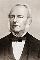
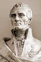
The fourth millennium problem got its name from the mathematicians Claude-Louis Navier (1785-1836), on the left, and George Gabriel Stokes (1819-1903), on the right. As a result of their research it was established that the motion of a viscous and incompressible fluid can be modelled using what we know today as the «Navier-Stokes equations». / Mètode

The equations of motion for a fluid were obtained by Leonhard Euler in the mid-eighteenth century. In essence, he did nothing else than applying the principle of conservation of mass and Newton’s second law to quite a rich collection of material parts of the fluid. We can identify a material part as the region of space it occupies at a given moment. But a moment later it will occupy a different one, that will depend on the motion of the fluid. More specifically, Euler considered infinitesimal material parts: for each time instant and around each point, he considered the matter contained within a cuboid of infinitesimal edges dx, dy, dz. This led him to the equations of motion in differential form.

The forces that affect a material part of the fluid are divided in two classes: those that act from a distance, such as gravity, and those that act by contact with the neighbouring material parts, like pressure. Euler considered both gravity and pressure, but not another contact force that is essential to deduce, for instance, that the water in our container will tend towards rest. For that we must include also viscosity, that can be understood as an internal friction that acts against the differences in velocity. Contact forces associated with viscosity were not suitably modelled until well into the nineteenth century. This was the (more or less independent) work of Claude Navier, Augustin Cauchy, Siméon Poisson, Adhémar Barré de Saint-Venant, and George Gabriel Stokes.

As a result of their research, it was established that the motion of a viscous and incompressible fluid in a closed and immobile container can be modelled by using what we know today as the «Navier-Stokes equations». In vector notation they can be written as follows:

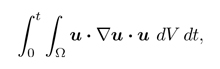
In principle there are two unknowns, velocity u and pressure p, which are functions of the position x and time t. Position x runs across the whole region Ω occupied by the fluid. Time t advances from 0 to +∞. To be precise, all the terms of equation 1 except the last one should be multiplied by the fluid’s density, but from now on we will assume that it is the same everywhere and that the units have been chosen so that its value is 1. There is also a parameter, v, which depends on the fluid and quantifies the degree of viscosity. The rest of the notation is common in vector calculus: ∇ = (∂/∂x,∂/∂y,∂/∂z) is the gradient operator, which we use formally as a vector that can be scalarly multiplied by another; in particular, ∇·u is the divergence of the vector field u, and u·∇ is what we call the advection operator; finally, Δ is the Laplace operator Δ = ∇·∇.

Equations 1 and 2 must be fulfilled at any point in the region Ω. On the other hand, equation 3 refers only to the surface ∂Ω that limits Ω: for a viscous fluid, velocity must vanish at any point of this surface. In the spirit of getting rid of certain complications caused by equation 3, we often consider also the case where Ω is the entire space, with no limiting surface. In this case, however, one usually adds either an asymptotic condition at infinity, or simply a finiteness condition for the total (kinetic) energy

(where u denotes the magnitude of the u vector), or perhaps a condition of spatial periodicity in three orthogonal directions; in the following explanation we will always assume some condition of this kind, even if we do not specify it. Finally, equation 4 specifies the initial state of motion of the fluid.

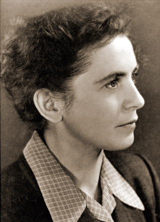
Despite belonging to a family persecuted by Stalin’s regime, Olga Ladyzhenskaya (1922-2004) became one of the most prominent figures in the soviet school of partial differential equations. Her favourite research topic was the mathematical theory of viscous incompressible fluids. / Images des Mathématiques

So, the question that was formulated above can now be expressed as follows: is it true that for each initial state u₀ there is a unique solution of the Navier-Stokes equations, and that it remains defined for arbitrarily large times? Next, we will examine the efforts that have been made to answer this question, mainly by Carl Oseen, Jean Leray, and Olga Ladyzhenskaya during the twentieth century.

Classical solutions

The existence and uniqueness of solutions of the Navier-Stokes equations for a given initial state can be studied by means of the method of successive approximations: starting from a first approximation, we can introduce it in the non-linear term of equation 1 –  the one containing (u·∇)u  – and try to solve the resulting equation so as to obtain a new approximation; then we can repeat the process with the result and so on in the hope that this process will take us closer and closer to the exact solution. Unlike equation 1, the one we use at each step of this iteration is linear (not homogeneous). Related to this, its solution can be expressed through an integral combination of certain special solutions that correspond to point-concentrated instantaneous impulses.

Following this path, Oseen and Leray managed to deal, among other cases, with the case where Ω is the entire space, for which those special solutions can be explicitly calculated. Leaving aside some technical details, the results they obtained are as follows:

a) If the time limit for which a solution is sought is small enough, then we have one solution and only one.

b) In general, the solution cannot be extended beyond a certain time T, which can be finite or infinite depending on the initial state.

c) If T is finite, then the solution develops singularities when t approaches T; in other words, there are points X of Ω where the velocity becomes arbitrarily large as we get closer to (X, T).

In fact, the method of successive approximations replaces the differential equations 1-4 by an integral equation. This equation allows us to see that, as long as there are no singularities, the obtained solutions are smooth functions, that is, they are infinitely differentiable, and fulfil the differential equations in the classical sense.

According to the contrapositive of (c), in order to ensure that the solution remains defined for arbitrarily large times, it suffices to obtain an upper bound on the magnitude that can reach the velocity vector. Related to this, it is not difficult to see that the total (kinetic) energy of the fluid decreases over time. Indeed, as observed by Stokes, multiplying equation 1 scalarly by u and integrating by parts, we obtain the so-called «energy equality»:

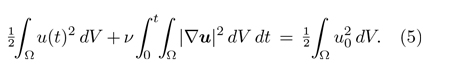
However, the fact that an integral is finite does not exclude the possibility that the integrand becomes infinite at some point. In other words, the inequality

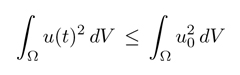
that follows from equation 5 is not enough to ensure that the solution is global in time.

Having said that, in the two-dimensional case (Ω ⊆ R²), the upper bound on

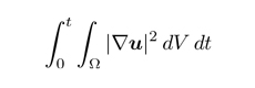
which also follows from equation 5 allows to derive the one mentioned above, thus guaranteeing that the solution remains defined for arbitrarily large times, whatever the initial state.

In contrast, in the three-dimensional case, the temporal globality of the solution has been obtained only in the case where the initial energy and velocities are small enough, or where the viscosity is large enough.

Singularities and turbulence

It is interesting to observe that, in practice, predictions become difficult precisely in the opposite conditions to those of the result we have just discussed; that is, for high velocities and low viscosities. Osborne Reynolds’s 1883 experiment on turbulence is very illustrative of this, since it shows clearly unpredictable spacetime developments taking place under these conditions.

All this leads to conjecturing that the solutions of the Navier-Stokes equations could indeed develop singularities, which would be related to complications when trying to make detailed predictions about turbulent motions.

At least, this was the opinion of Oseen, as well as Leray and Ladyzhenskaya. The following quotations can be found in Mora (2008).

In 1910, Oseen already expressed himself in the following terms:

According to our theory, therefore, it seems likely that irregularities may arise at the interior of an incompressible viscous, even when both the external forces and the initial motion are completely regular.

In his 1927 book he explicitly mentioned the possible relationship between singularities and turbulence:

If singularities can arise, then we must obviously distinguish between two kinds of motion of a viscous fluid: the regular motions, i.e., motions without singularities, and the irregular motions, i.e., motions with singularities. On the other hand, hydraulics is already distinguishing between two kinds of motions: the laminar motions and the turbulent ones. This leads us to conjecturing that the «laminar» motions of the experiments correspond to the «regular» motions of the theory, and the «turbulent» motions of the experiments correspond to the «irregular» motions of the theory. Only further researches can decide whether this conjecture is true.

Regarding Leray, it suffices to say that he adopted the name «turbulent solutions» to refer a the generalised notion of solution that, as we will see below, could extend beyond some types of singularities. In addition, he also supported the view that solutions could develop singularities:

However, it does not seem possible to deduce from this fact that the motion itself remains regular; I even pointed out a reason which makes me believe in the existence of motions that become irregular after a finite time; unfortunately, I have failed to construct an example of such a singularity.

Finally, regarding Ladyzhenskaya we quote the following text about the lack of uniqueness that, as we will see below, could occur after the singularities:

But one cannot exclude the possibility that at some moment this smoothness will be destroyed. […] At such catastrophic moments the solution may branch. […] We think that such a branching of the solution is possible in the Navier-Stokes equations.

Globally dissipative weak solutions

Faced with the possibility that the solutions of the Navier-Stokes equations might develop singularities, it is natural to wonder: can the Navier-Stokes equations make sense for velocity fields that contain singularities?

Indeed, the presence of a singularity implies that the velocity is not well defined everywhere, even less so for its derivatives, so the different terms of the differential equations that should determine the future motion of the fluid stop making sense.

In this connection, Oseen already observed that the integral equation of the method of successive approximations can still make sense in the presence of singularities. Not only that; in fact, he proved that this integral equation could be obtained directly from the equations that balance out mass and momentum for a finite part of material (not infinitesimal, as in Euler’s case).

Notably, one of the intermediate steps of this deduction corresponds to a generalised concept of solution that was later adopted by Leray and is currently a standard tool in the study of partial differential equations. These solutions in a more general sense are called «weak solutions». Thus, the question that we were posing has a positive answer.

On the other hand, it is also true that the Navier-Stokes equations assume that friction forces depend linearly on the spatial derivatives of velocity, which might not be true for high values of these derivatives. This leads to replacing the equations with some variations that do admit global solutions for any initial state, and studying the limit of these solutions for a particular initial state as we get closer and closer to the Navier-Stokes equations.

When developing this idea, Leray was unable to guarantee a single limit for the entire sequence of perturbed solutions. He only proved the existence of subsequences that converge in a particular sense, with limits that might change from one subsequence to another. Anyway, each of these limits is guaranteed to be a weak global solution of the Navier-Stokes equations for the given initial state.

The way Leray modified the equations had the property that all the perturbed solutions fulfilled the energy equality (equation 5). Even so, the sense in which the mentioned subsequences converge is too weak to guarantee that the limit fulfils the same equality. What one can deduce, though, is that the obtained weak solutions comply with the so-called «energy inequality», where the sign «=» in equation 5 is replaced by «≤»:

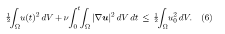
Note that this inequality is not deduced from the fact that u is a solution in the weak sense! Because there is no such deduction. More specifically, the path we followed for classical solutions – the Stokes calculations we indicated in the third section – is not valid, since it involves the integral

which does not make sense in the low-regularity conditions assumed by the concept of weak solution.

In view of this, and of the importance of energy inequalities, it makes sense to introduce a new concept of solution that explicitly asks for this inequality to hold, besides fulfilling the equation in the weak sense. These are what Leray called «turbulent solutions». Instead, we will call them «globally dissipative solutions».

Locally dissipative weak solutions

Remember that regular solutions fulfil equation 6 as an equality. This equality quantifies how energy decreases due to viscosity. Therefore, when we ask a weak solution to fulfil inequality 6, what we are saying is: if singularities involve a deviation from the energy equality, this deviation must be in the direction of producing an additional energy decrease.

This restriction is in line with the second law of thermodynamics, which in our context refers to the dissipation of macroscopic kinetic energy by its conversion into microscopic energy. However, the second law must be fulfilled not only in the fluid as a whole, but also in any part of it.

This naturally leads to a more restrictive concept of solution that includes a local version of the energy inequality. These solutions, which can be called «locally dissipative solutions», were introduced in 1977 by Vladimir Scheffer. He proved that the weak solutions obtained by Leray’s method of perturbation fulfil this condition, and used this fact to bound the dimension of the set of singularities. Such results were later improved by Luis Caffarelli, Robert Kohn, and Louis Nirenberg, among others.

Conclusion

«Fluid mechanics is not so different from celestial mechanics regarding determinism»

So, the problem is still, essentially, the one we laid out in the second section of this document («The equations of motion»); that is, whether or not there is a unique solution for each initial state, and whether it will remain defined for arbitrarily large times. But we have also seen that the concept of solution admits of certain variations, so that now it is appropriate to consider it also as part of the answer.

We have to admit that this problem is not exactly that of the Clay Institute prize. The latter refers to the conjecture we formulated in the fourth section («Singularities and turbulence»): clarifying – with a demonstration or a counterexample – whether regular solutions remain defined for arbitrarily large times or whether singularities can develop in finite time.

A fluid consists of a large number of molecules that collide very frequently with each other. In the picture, smoke ascending with a horizontal current. / Graham Jeffery

Note that an example of a solution that develops singularities would answer this, but not the fundamental one of determinism, since it might still happen that the solution admits only one continuation within the class of locally dissipative solutions.

Going back to the comparison we made in the introduction, the fact is that celestial mechanics is neither completely deterministic in the sense that we are considering: even in the ideal case of point bodies, collisions cannot be ruled out; and, in general, triple collisions admit of multiple ways for the motion to be continued.

Therefore, in the end, fluid mechanics is not so different from celestial mechanics regarding determinism. After all, a fluid is consists of a large number of molecules that collide very frequently with each other.

REFERENCES

Mora, X. (2008). Les equacions de Navier-Stokes. Un repte al determinisme newtonià. Butlletí de la Societat Catalana de Matemàtiques, 23, 53–120. doi: 10.2436/20.2002.01.12
Seregin, G., & Šverák, V. (2017). On global weak solutions to the Cauchy problem for the Navier-Stokes equations with large L3-initial data. Nonlinear Analysis, 154, 269–296. doi: 10.1016/j.na.2016.01.018